基础算法优化——Fast Modular Multiplication

1. 引言

Yuval Domb 2022年论文《Fast Modular Multiplication》

模乘可以说是任何密码系统中计算量最大的算术原语。本文提出了一种高效、硬件友好的算法，据作者所知，该算法优于迄今为止的算法。

标准的modulo-prime multiplication problem in ${\mathbb{F}}_s$表示为：
$$\begin{array}{c}r=a\cdot b\mathrm{mod}s\end{array}$$
其中 $a,b,s\in {\mathbb{F}}_s$，$s$为素数，并利用标准$\mathbb{Z}$-algebra。
等价为：
$$\begin{array}{c}a\cdot b=l\cdot s+r\end{array}$$
其中，$l\in \mathbb{Z}$，使得 $0\le r<s$。

本文主要为（1）中计算提供了一种高效、硬件友好的快速计算方法。

将所有变量以$d$-进制来表示，其中${\mathbb{F}}_s$内的每个元素都以$n$个digits来表示，有：
$$\begin{array}{c}n=\lceil {\log }_{d}s\rceil \end{array}$$

接下来，简单地令$d=2$，所有元素以二进制来表示。

尽管本文重点关注modulo-prime multiplication，但可将其推广到任意$a\mathrm{mod}s$运算，其中$a<s^2$，$s$可为素数或非素数的任意值。

2. 本文主要贡献

本文主要展现了，如何将：

• Barrett Reduction算法（具体见Barrett 1987年论文《Implementing the rivest shamir and adleman public key encryption algorithm on a standard digital signal processor》）
• 与 好的参数选择
• 以及 简单的bounding技术

结合，用于求取quotient $l$的近似值，近视精度为一个小的constant error，该constant error与$n$无关（无论$n$值大小）。

令人惊讶的是，最终的reduction算法与Montgomery的Modular-Multiplication算法（见Montgomery 1985年论文《 Modular multiplication without trial division》）类似，但是本文最终的reduction算法不需要coordinate translation。

本文的bounding技术可用于进一步降低特定感兴趣场景的计算复杂度（知识需要增加constant error），本文不展开。

3. Reduction Scheme

3.1 假设 $l$ 为近似已知

假设 $l$ 为近似已知，将其近似值表示为 $\hat{l}$，使得：
$$\begin{array}{c}l-\lambda \le \hat{l}\le l\end{array}$$
其中$\lambda =O(1)$为一个已知的constant。

若$\lambda =0$，则显然有：
$$\begin{array}{c}ab[2n-1:0]-\hat{l}s[2n-1:0]=r[n-1:0]\end{array}$$
其中[]中括号内的值表示了bit locations和sizes。

注意，当$\lambda =0$时，可推测余数$r$最大长度为 $n$ bits，使得等式（5）中右侧值的剩余最高有效位（ms (most-significant) bits）必须为$0$。

通过简单的bit操作，可以long addition表示为：

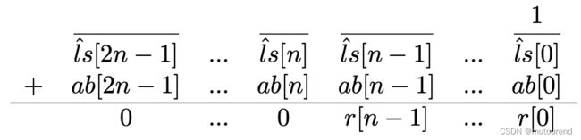
其中，上横杠表示的是bit-inversion运算符，横岗上的$1$表示为初始carry bit。
不过，对上面的long addition表示仔细观察可知，仅需要 $ab[n-1:0]$ 和 $\hat{l}s[n-1:0]$ 来完成该计算，从而可节约近一半的计算量。最终的adder为a fixed width adder——即，$n+n\to n$。这意味着可忽略 ms bits（最高有效位）的任何溢出。可将其等价为a fixed-width subtractor——即，$n-n\to n$，可将其结果看成是unsigned integer。

将生成以上乘积的multiplier表示为$n\times n\to n_{\text{lsb}}$，其中$n_{\text{lsb}}$是指该full product的$n$个least-significant bits。$a\cdot b$和$\hat{l}\cdot s$都可通过$n\times n\to n_{\text{lsb}}$来生成。
此外，若$s$为constant，$\hat{l}\cdot s$可通过一个constant $n\times n\to n_{\text{lsb}}$ multiplier来生成。

当$\lambda \ne 0$时：
$$\begin{array}{c}ab-\hat{l}s=r+\lambda s\end{array}$$
此时，用于表示等式（5）中右侧值所需的number of bits为：
$$\begin{array}{c}\lceil {\log }_2(r+\lambda s)\rceil \le n+\lceil {\log }_2\frac{r+\lambda s}{s}\rceil \le n+\lceil {\log }_2(1+\lambda )\rceil \end{array}$$
因此，若$\lambda =1$，则仅需要额外再增加$1$个bit来表示。

3.2 使用Barrett Reduction算法求$l$的近似值

采用Barrett的modular reduction算法对$l$求近似值为：
$$\begin{array}{c}l=\lfloor \frac{ab}{s}\rfloor =\underset{k\to \infty }{\lim }\frac{ab\cdot m(k)}{2^{k+n}}\end{array}$$
其中：
$$\begin{array}{c}m(k)=\lfloor \frac{2^{k+n}}{s}\rfloor <2^{k+1}\end{array}$$
为a function of the $k$，最多有$k+1$ bits，为公式（8）的lower-bound approximator。对于有限的$k$值，该approximation error为：
$$\begin{array}{c}e(k)\equiv \frac{1}{s}-\frac{m(k)}{2^{k+n}}<2^{-(k+n)}\end{array}$$
其中，可检查二进制表示的左右项的最大差异来派生出该upper-bound。从而有approximation error on $l(k)$为：
$$\begin{array}{c}e(l,k)\equiv \frac{ab}{s}-\frac{ab\cdot m(k)}{2^{k+n}}<2^{2n}\cdot 2^{-(k+n)}=2^{n-k}\end{array}$$
若$k\ge n$，则该approximation error最多为$1$。

3.3 参数选择 以及 error bounding

选择$k=n$（即$m(n)<2^{n+1}$），则对$l$的近似值为：
$$\begin{array}{c}{\hat{l}}_0=\lfloor \frac{abm}{2^{2n}}\rfloor \end{array}$$
$$\begin{array}{c}e({\hat{l}}_0)<1\end{array}$$
其中multiplication为$n\times n\times (n+1)\to (n+1{)}_{\text{msb}}$，且approximation error遵循（11）。

分两个阶段来实现以上multiplication：

• 1）首先，假设有$ab[2n-1:0]$，按如下方式计算multiplication：
  $$\begin{array}{c}\frac{abm}{2^{2n}}=\frac{ab[2n-1:n]\cdot m}{2^n}+\frac{ab[n-1:0]\cdot m}{2^{2n}}\end{array}$$
  $$\begin{array}{c}<\frac{ab[2n-1:n]\cdot m}{2^n}+2\end{array}$$
  其中最右侧项trivially upper-bounded by $2$。
• 2）从而对$l$的近似变为：
  $$\begin{array}{c}{\hat{l}}_1=\lfloor \lfloor \frac{ab}{2^n}\rfloor \cdot \frac{m}{2^n}\rfloor \end{array}$$
  $$\begin{array}{c}e({\hat{l}}_1)<3\end{array}$$
  其中，最里侧的multiplication为$n\times n\to n_{\text{msb}}$，最外侧的constant multiplication为$n\times (n+1)\to (n+1{)}_{\text{msb}}$，approximation error由（13）和（15）中的最右侧项 之和 upper-bounded。

注意，由于$m(n)$ is typically very close to $2^n$，且$n$通常很大，无需额外增加bits来表示（17）中的constant error，即$n+1$ bits就足够了。
尽管如此，必须为每个特定setup检查并排除溢出的边界情况。

3.4 总体算法

以下为hardware-optimized modular multiplier结构图，假定了$s$和$m$为已知的constants，使用${\hat{l}}_1$来表示$l$的近似值。

注意，最左侧的multiplication module独立于reduction logic，使得该circuit的remainder可generalized beyond multiplication reduction。

3.5 举例

3.5.1 以$n=16$举例

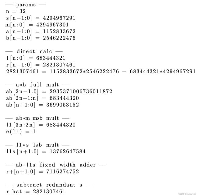
3.5.2 以$n=32$举例

3.5.3 例外情况

当$s=65717,a=65535,b=65631$时，真实$l$值应为$\lfloor \frac{ab}{s}\rfloor =65449$。而根据本文算法获得近似值 ${\hat{l}}_1=65546$，此时，error $e({\hat{l}}_1)$的值为$3$。
不过，对于prime $s$，这样的例外情况并不多，对于大多数的primes，最大可能error将不会超过$2$。