365天深度学习训练营-第T4周:猴痘病识别
- 本文为365天深度学习训练营 中的学习记录博客
- 原作者:K同学啊
我的环境:
- 语言环境:Python3.10.7
- 编译器:VScode
- 深度学习环境:TensorFlow2
一、前期工作:
1、导入数据集
from tensorflow import keras
from tensorflow.keras import layers, models
import os, PIL, pathlib
import matplotlib.pyplot as plt
import tensorflow as tf

data_dir = "D:\T4猴痘病"
data_dir = pathlib.Path(data_dir)

#查看图片数量
image_count = len(list(data_dir.glob("*/*.jpg")))
print(image_count)![]()
Monkeypox = list(data_dir.glob("Monkeypox/*.jpg"))
image_path = str(Monkeypox[0])

# Open the image using PIL
image = PIL.Image.open(image_path)

# Display the image using matplotlib
plt.imshow(image)
plt.axis("off")
plt.show()
2. 数据预处理
2.1设置图片格式
batch_size = 32
img_height = 224
img_width = 224
2.2划分训练集
train_ds = tf.keras.preprocessing.image_dataset_from_directory(
    data_dir,
    validation_split = 0.2,
    subset = "training",
    seed = 123,
    image_size = (img_height, img_width),
    batch_size = batch_size
)tf.keras.preprocessing.image_dataset_from_directory函数从目录中创建图像数据集。该函数可以方便地从磁盘上的文件夹中加载图像数据并进行预处理。
参数解释如下:
data_dir: 字符串,指定包含图像数据的目录路径。validation_split: 浮点数,指定验证集的比例。例如,设置为0.2表示将20%的数据用作验证集,剩余80%用作训练集。subset: 字符串,指定要创建的子集类型。在这里,设置为"training"表示创建训练集。seed: 整数,用于随机数生成的种子,以确保结果可重复。image_size: 元组,指定图像的目标尺寸。例如,(img_height, img_width)表示将图像调整为给定的高度和宽度。batch_size: 整数,指定每个批次中的图像数量。
运行结果:
2.3划分验证集
val_ds = tf.keras.preprocessing.image_dataset_from_directory(
    data_dir,
    validation_split = 0.2,
    subset = "validation",
    seed = 123,
    image_size = (img_height, img_width),
    batch_size = batch_size
)
运行结果:
2.4查看标签
class_names = train_ds.class_names
print(class_names)
运行结果:
2.5数据可视化
plt.figure(figsize = (20, 10))#创建一个图形对象,并指定其大小为20x10英寸

for images, labels in train_ds.take(1):#遍历train_ds数据集中的第一个批次,每个批次包含一批图和对应的标签。这里使用take(1)函数从数据集中获取一个批次。
  for i in range(20):
#在图形对象中创建一个子图,这里的子图是一个5x10的网格,并将当前子图设置为第i+1个位置。
    plt.subplot(5, 10, i + 1)
#使用Matplotlib的imshow函数显示当前图像。images[i]是当前图像的张量表示,使用.numpy()将其转换为NumPy数组,并使用.astype("uint8")将数据类型转换为uint8以便显示。
    plt.imshow(images[i].numpy().astype("uint8"))
#为当前图像设置标题,标题内容是通过索引labels[i]从class_names列表中获取的类别名称。
    plt.title(class_names[labels[i]])
#坐标轴显示
    plt.axis("off")
plt.show()代码使用Matplotlib库绘制训练数据集train_ds中的前20张图像,并显示其对应的标签(类名)。代码中定义的class_names是一个包含数据集类别名称的列表。
注意,这里使用了train_ds.take(1)来从train_ds数据集中取出第一个批次的图像和标签。train_ds是一个tf.data.Dataset对象,它包含了经过预处理和批量处理的训练图像数据。
2.6检查数据
for image_batch, labels_batch in train_ds:
  print(image_batch.shape)
  print(labels_batch.shape)
  break
2.7配置数据集
AUTOTUNE = tf.data.AUTOTUNE

train_ds = train_ds.cache().shuffle(1000).prefetch(buffer_size = AUTOTUNE)
val_ds = val_ds.cache().prefetch(buffer_size = AUTOTUNE)
shuffle():打乱数据
具体来说,shuffle(1000) 的作用是将数据集中的样本顺序进行随机打乱,以增加样本之间的独立性,并减少模型训练时对数据的记忆性。
参数 1000 表示要在数据集中创建一个缓冲区,其中包含 1000 个样本。在进行数据读取时,会从缓冲区中随机选择样本,并将其作为当前的批次。每个样本在缓冲区中的位置是随机的,并且会随着每个批次的读取而不断更新。
prefetch():预取数据,加速执行
prefetch()功能详细介绍: CPU正在准备数据时,加速器处于空闲状态。相反,当加速器正在训练模型时,CPU处于空闲状态。因此,训练所用的时间是CPU预处理时间和加速器训练时间的总和。
prefetch()将训练步骤的预处理和模型执行过程重叠到一起。当加速器正在执行第N个训练步时,CPU正在准备第N+1步的数据。这样做不仅可以最大限度地缩短训练的单步用时(而不是总用时),而且可以缩短提取和转换数据所需的时间。如果不使用prefetch() ,CPU和GPU/TPU在大部分时间都处于空闲状态。
cache():将数据缓存到内存当中
三、搭建CNN网络
#设置Sequential模型,创建神经网络
model = models.Sequential([
layers.experimental.preprocessing.Rescaling(1./255,input_shape=(img_height,img_width,3)),
#设置二维卷积层1,设置32个3*3卷积核,activation参数将激活函数设置为ReLU函数
#input_shape设置图形的输入形状
layers.Conv2D(32, (3, 3), activation='relu', input_shape=(img_height, img_width, 3)),
#池化层1,2*2采样
layers.AveragePooling2D(2*2),
#设置二维卷积层2,设置64个3*3卷积核,激活函数设置为ReLU函数
layers.Conv2D(64, (3, 3), activation='relu'),
#池化层2,2*2采样
layers.AveragePooling2D((2, 2)),
#设置停止工作概率,防止过拟合
layers.Dropout(0.3),
#Flatten层,用于连接卷积层与全连接层
layers.Flatten(),
#全连接层,特征进一步提取,64为输出空间的维数(神经元),激活函数为ReLU函数
layers.Dense(128,activation='relu'),
#输出层,4为输出空间的维数
layers.Dense(4)
])
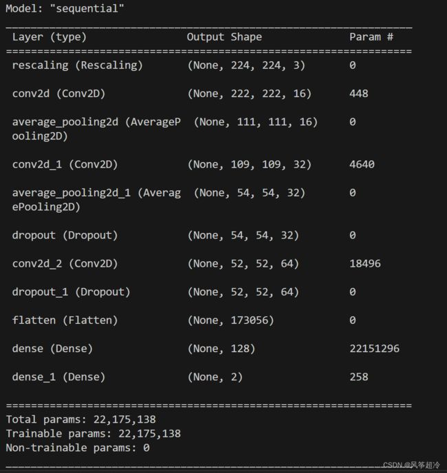
#打印网络结构
model.summary()运行结果:
四、编译
在准备对模型进行训练之前,还需要再对其进行一些设置 。以下内容是在模型的编译步骤中添加的:
●损失函数(loss) :用于衡量模型在训练期间的准确率。
●优化器(optimizer) :决定模型如何根据其看到的数据和自身的损失函数进行更新。
●指标(metrics) :用于监控训练和测试步骤。以下示例使用了准确率,即被正确分类的图像的比率。
#设置优化器
opt = keras.optimizers.Adam(learning_rate=0.001)
model.compile(
    #设置优化器为Adam优化器
    optimizer = opt,
    #设置损失函数为交叉熵损失函数
    #from_logits为True时,会将y_pred转化为概率
    loss = keras.losses.SparseCategoricalCrossentropy(from_logits=True),
    #设置性能指标列表,将在模型训练时对列表中的指标进行监控
    metrics = ['accuracy']
)
五、训练模型
from tensorflow.keras.callbacks import ModelCheckpoint

epochs = 50

checkpointer = ModelCheckpoint(
    'best_model.h5',
    monitor = 'val_accuracy',
    verbose = 1,
    save_best_only = True,
    save_weights_only = True
)

history = model.fit(
    train_ds,
    validation_data = val_ds,
    epochs = epochs,
    callbacks = [checkpointer]
)
运行结果:
六、模型评估
6.1Loss和Acc图
loss = history.history['loss']
val_loss = history.history['val_loss']

acc = history.history['accuracy']
val_acc = history.history['val_accuracy']

epochs_range = range(len(loss))

plt.figure(figsize = (12, 4))

plt.subplot(1, 2, 1)
plt.plot(epochs_range, acc, label = "Training Acc")
plt.plot(epochs_range, val_acc, label = "Validation Acc")
plt.legend(loc = 'lower right')
plt.title("Training And Validation Acc")

plt.subplot(1, 2, 2)
plt.plot(epochs_range, loss, label = "Training Loss")
plt.plot(epochs_range, val_loss, label = "Validation Loss")
plt.legend(loc = 'upper right')
plt.title("Training And Validation Loss")

plt.show()
上述代码是用于绘制训练和验证准确率以及训练和验证损失随着训练周期的变化趋势的图表。
`acc = history.history['accuracy']`:从训练历史记录中获取训练准确率的数值列表。
`val_acc = history.history['val_accuracy']`:从训练历史记录中获取验证准确率的数值列表。
`loss = history.history['loss']`:从训练历史记录中获取训练损失的数值列表。
`val_loss = history.history['val_loss']`:从训练历史记录中获取验证损失的数值列表。
`epochs_range = range(epochs)`:创建一个表示训练周期范围的迭代器,其中 `epochs` 是训练周期的总数。
接下来,使用 `matplotlib.pyplot` 绘制图表:
`plt.figure(figsize=(12, 4))`:创建一个图表对象,设置图表的大小为 (12, 4)。
`plt.subplot(1, 2, 1)`:创建一个子图,表示第一个子图,用于绘制准确率。
`plt.plot(epochs_range, acc, label='Training Accuracy')`:绘制训练准确率随着训练周期的变化曲线。
`plt.plot(epochs_range, val_acc, label='Validation Accuracy')`:绘制验证准确率随着训练周期的变化曲线。
`plt.legend(loc='lower right')`:显示图例,并设置其位置在右下角。
`plt.title('Training and Validation Accuracy')`:设置子图的标题为 "Training and Validation Accuracy"。
`plt.subplot(1, 2, 2)`:创建一个子图,表示第二个子图,用于绘制损失。
`plt.plot(epochs_range, loss, label='Training Loss')`:绘制训练损失随着训练周期的变化曲线。
`plt.plot(epochs_range, val_loss, label='Validation Loss')`:绘制验证损失随着训练周期的变化曲线。
`plt.legend(loc='upper right')`:显示图例,并设置其位置在右上角。
`plt.title('Training and Validation Loss')`:设置子图的标题为 "Training and Validation Loss"。
`plt.show()`:显示图表。
运行结果:
6.2指定结果进行预测
model.load_weights('best_model.h5')

from PIL import Image
import numpy as np

img = Image.open("D:/T4MonkeyPox/Monkeypox/M01_02_06.jpg")

image = tf.image.resize(img, [img_height, img_width])

img_array = tf.expand_dims(image, 0)


predictions = model.predict(img_array)
#这个函数用于对输入图像进行分类预测。它使用已经训练好的模型来对输入数据进行推断,并输出每个类别的概率分布。
print("预测结果为:", class_names[np.argmax(predictions)])
model.load_weights('best_model.h5')
代码用于加载之前训练中保存的最佳模型权重。'best_model.h5' 指的是之前保存的模型权重文件路径和名称。这样可以避免从头开始训练模型,直接使用已经训练好的最佳模型进行预测的工作。
img = Image.open("D:/T4MonkeyPox/Monkeypox/M01_02_06.jpg")
代码用于使用 PIL 库中的 Image.open() 方法打开一张待预测的图片。
image = tf.image.resize(img, [img_height, img_width])
这个函数调整输入图像的大小以符合模型的要求。
在这个例子中,使用 TensorFlow 的 tf.image.resize() 函数将图像缩放为指定大小,其中 img_height 和 img_width 是指定的图像高度和宽度。
img_array = tf.expand_dims(image, 0)
这个函数将输入图像转换为形状为 (1, height, width, channels) 的四维数组,
其中 height 和 width 是图像的高度和宽度,channels 是图像的通道数(例如 RGB 图像有 3 个通道)。这里使用 TensorFlow 的 tf.expand_dims() 函数来扩展图像数组的维度,以匹配模型的输入格式。
image 是一个二维图片张量,它的形状是 (height, width, channels)。其中 height 和 width 分别为图片的高度和宽度,channels 为图片的颜色通道数。0 是一个整数值,它指定在哪个维度上扩展此张量,这里表示在最前面(第一个)的维度上扩展。因此,函数的作用是将输入张量 image 在最前面添加一个额外的维度(batch_size),生成一个四维张量。
tf.expand_dims(input, axis)
其中 input 表示要扩展的输入张量,axis 表示要在哪个维度上进行扩展。在这个例子中,input 是变量 image,axis 是 0。
print("预测结果为:", class_names[np.argmax(predictions)])
将模型输出的概率分布转换为最终预测结果。
具体来说,使用 np.argmax() 函数找到概率最大的类别索引,然后使用该索引在 class_names 列表中查找相应的类别名称,并输出预测结果。
运行结果:
七、完整代码
from tensorflow import keras
from tensorflow.keras import layers, models
import os, PIL, pathlib
import matplotlib.pyplot as plt
import tensorflow as tf

data_dir = "D:\T4MonkeyPox"
data_dir = pathlib.Path(data_dir)

image_count = len(list(data_dir.glob("*/*.jpg")))

Monkeypox = list(data_dir.glob("Monkeypox/*.jpg"))

batch_size = 32
img_height = 224
img_width = 224

train_ds = tf.keras.preprocessing.image_dataset_from_directory(
    data_dir,
    validation_split = 0.2,
    subset = "training",
    seed = 123,
    image_size = (img_height, img_width),
    batch_size = batch_size
)

val_ds = tf.keras.preprocessing.image_dataset_from_directory(
    data_dir,
    validation_split = 0.2,
    subset = "validation",
    seed = 123,
    image_size = (img_height, img_width),
    batch_size = batch_size
)

class_names = train_ds.class_names

plt.figure(figsize = (20, 10))


AUTOTUNE = tf.data.AUTOTUNE

train_ds = train_ds.cache().shuffle(1000).prefetch(buffer_size = AUTOTUNE)
val_ds = val_ds.cache().prefetch(buffer_size = AUTOTUNE)

num_classes = 2

model = models.Sequential([
    layers.experimental.preprocessing.Rescaling(1. / 255, input_shape = (img_height, img_width, 3)),


    layers.Conv2D(16, (3, 3), activation = 'relu', input_shape = (img_height, img_width, 3)),
    layers.AveragePooling2D((2, 2)),
    layers.Conv2D(32, (3, 3), activation = 'relu'),
    layers.AveragePooling2D((2, 2)),
    layers.Dropout(0.3),
    layers.Conv2D(64, (3, 3), activation = 'relu'),
    layers.Dropout(0.3),

    layers.Flatten(),
    layers.Dense(128, activation = 'relu'),
    layers.Dense(num_classes)
])

#设置优化器
opt = keras.optimizers.Adam(learning_rate=0.001)
model.compile(
    #设置优化器为Adam优化器
    optimizer = opt,
    #设置损失函数为交叉熵损失函数
    #from_logits为True时,会将y_pred转化为概率
    loss = keras.losses.SparseCategoricalCrossentropy(from_logits=True),
    #设置性能指标列表,将在模型训练时对列表中的指标进行监控
    metrics = ['accuracy']
)

from tensorflow.keras.callbacks import ModelCheckpoint

epochs = 50

checkpointer = ModelCheckpoint(
    'best_model.h5',
    monitor = 'val_accuracy',
    verbose = 1,
    save_best_only = True,
    save_weights_only = True
)

history = model.fit(
    train_ds,
    validation_data = val_ds,
    epochs = epochs,
    callbacks = [checkpointer]
)

loss = history.history['loss']
val_loss = history.history['val_loss']

acc = history.history['accuracy']
val_acc = history.history['val_accuracy']

epochs_range = range(len(loss))

plt.figure(figsize = (12, 4))

plt.subplot(1, 2, 1)
plt.plot(epochs_range, acc, label = "Training Acc")
plt.plot(epochs_range, val_acc, label = "Validation Acc")
plt.legend(loc = 'lower right')
plt.title("Training And Validation Acc")

plt.subplot(1, 2, 2)
plt.plot(epochs_range, loss, label = "Training Loss")
plt.plot(epochs_range, val_loss, label = "Validation Loss")
plt.legend(loc = 'upper right')
plt.title("Training And Validation Loss")

plt.show()

model.load_weights('best_model.h5')

from PIL import Image
import numpy as np

img = Image.open("D:/T4MonkeyPox/Monkeypox/M01_02_06.jpg")

image = tf.image.resize(img, [img_height, img_width])

img_array = tf.expand_dims(image, 0)

predictions = model.predict(img_array)

print("预测结果为:", class_names[np.argmax(predictions)])