Automatic Differentiation
For beginners, the most daunting aspect of deep learning algorithms is perhaps Back-Propagations (BP) which require derivations of some highly complex mathematical expressions.
Luckily when actually implementing BP, we do not have to rely on smmary symbolic expressions at all and can simply use the trick call Automatic Differentiation (AD), or Autodiff.
Resources:
1. introduction and brief overview from wiki: https://en.wikipedia.org/wiki/Automatic_differentiation
2. an article with more detail and step-by-step example: https://marksaroufim.medium.com/automatic-differentiation-step-by-step-24240f97a6e6
3. a lecture slide with advanced examples: https://www.cs.toronto.edu/~rgrosse/courses/csc321_2018/slides/lec10.pdf
4. an academic survey of AD: https://www.jmlr.org/papers/volume18/17-468/17-468.pdf
Overview
From Wikipedia, the free encyclopedia
In mathematics and computer algebra, automatic differentiation (auto-differentiation, autodiff, or AD), also called algorithmic differentiation, computational differentiation,[1][2] is a set of techniques to evaluate the partial derivative of a function specified by a computer program.
Automatic differentiation exploits the fact that every computer calculation, no matter how complicated, executes a sequence of elementary arithmetic operations (addition, subtraction, multiplication, division, etc.) and elementary functions (exp, log, sin, cos, etc.). By applying the chain rule repeatedly to these operations, partial derivatives of arbitrary order can be computed automatically, accurately to working precision, and using at most a small constant factor of more arithmetic operations than the original program.
how AD compares to Symbolic Differentiation and Numerical Differentiation:
Automatic differentiation is distinct from symbolic differentiation and numerical differentiation. Symbolic differentiation faces the difficulty of converting a computer program into a single mathematical expression and can lead to inefficient code. Numerical differentiation (the method of finite differences) can introduce round-off errors in the discretization process and cancellation. Both of these classical methods have problems with calculating higher derivatives, where complexity and errors increase. Finally, both of these classical methods are slow at computing partial derivatives of a function with respect to many inputs, as is needed for gradient-based optimization algorithms. Automatic differentiation solves all of these problems.
the basis for AD is chain rule, recall:
Usually, two distinct modes of automatic differentiation are presented.
- forward accumulation (also called bottom-up, forward mode, or tangent mode)
- reverse accumulation (also called top-down, reverse mode, or adjoint mode)
we see that forward acc. is performed per independent variable x, and reverse acc. is performed per function (y); let's call each execution a "sweep", and
note that for most machine learning algorithms, BP for error propagation usually works better with the reverse acc. since we are mapping a huge pool of parameters to a small set of decision options.
Some Details and Step-by-Step
from resource 2, with some comments.
Symbolic Differentiation
Symbolic differentiation works by breaking apart a complex expression into a bunch of simpler expressions by using various (basic calculus) rules — very similar to a compiler.
The main issue with symbolic differentiation is that in simplifying the expression we could instead end up with an exponentially large expression to evaluate which will be prohibitively slow — O(2^n)
==> as humans, we usually deal with exploding terms by reduction methods or observing patterns, i.e. using series summation, or recursion rules; this is obviously unsuitable for generalized programs.
Numeric Differentiation
Symbolic differentiation isn’t used much in practice but it’s great to prototype with.
Numeric Differentiation is far more popular and effectively the default way to compute derivatives in most applications. The usual formula is below
This equation is derived via the famous Taylor Series expansion which lets you write a function in terms of its higher order derivatives.
The main issue with numeric differentiation is that if ϵ is too small, computers will end up facing floating point errors and give incorrect results! If ϵ is too large then the result will be an approximation. It’s also slow O(n).
==> again, as human, we deal with inifinity by mathematical observations, which cannot be transported to generalized programs.
Automatic Differentiation
Automatic Differentiation gives exact answers in constant time (to the original function). However, it does require introducing some unfamiliar math but it’s really simple after you skim it once.
Before we introduce Automatic Differentiation we need to talk about Dual Numbers.
Dual numbers
Dual numbers are numbers of the form a + bϵ where ϵ² = 0
or more technically, from wiki:
Dual numbers look like complex numbers if you replace i² = -1 by ϵ² = 0 but they’re unrelated so don’t let the similarity distract you.
Suppose you have two dual numbers a + bϵ and c + dϵ you can do arithmetic expressions on them
If you add 2 dual numbers you get a dual number
![]()
If you multiply 2 dual numbers you get a dual number
![]()
Addition and Multiplication in of themselves are not particularly useful but the power of dual numbers shines when we take a look a the Taylor series expansion of a function about a dual point instead of a regular point like what we saw in numeric optimization.
Taylor Series about a Dual Point
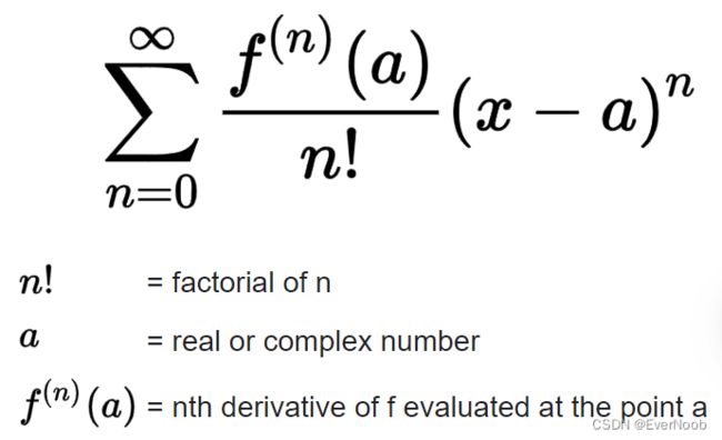
Plain Taylor series approximates a function f about a point a by using all its higher order derivatives.
the expression above is wrong, see Wolfram:
and full summation expression is:
Instead of approximating f about a real number a
We will approximate f about a real number a + ϵ
==> to end up with expression below, the above approximation must be expanding f(x) at around a, while assuming x = a + epsilon, where epsilon approaches 0.
We end up with the expression
Dual numbers have the convenient property that ϵ² = 0 which means ϵ³, ϵ⁴ … all = 0.
So the expression simplifies to
So if you evaluate a function f at a dual number a + ϵ you evaluate the function AND get its derivative for free
The solution we obtained is also EXACT because we are not ignoring the higher order derivatives like in numeric differentiation but we are eliminating them.
The solution can be computed FAST because we are just evaluating a function and not dealing with infinite sums or any such nonsense. Symbolic differentiation is also exact but it’s slow because you need to expand out an exponential number of expressions to evaluate it
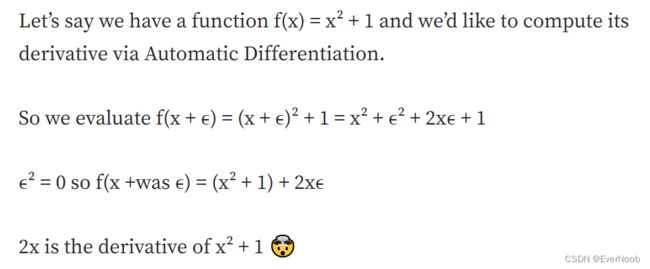
A simple example
==> we are only interested in the real coefficient.
While the above algorithm works it suffers from the same performance issues as Symbolic Differentiation where we need to expand out a potentially exponentially sized expression.
So next we’ll go over the two main algorithms for Automatic Differentiation forward mode and Reverse Mode Automatic Differentiation with an example borrowed from Automatic Differentiation in Machine Learning: a Survey
Forward Mode Differentiation
The first step in both the forward and Reverse Mode AD algorithms is to represent a function as a computational graph, also called a Wengert list.
Each node v in this list will represent an intermediate result of the computation. The intermediate results can then be assembled using the chain rule to get the final derivative we’re looking for.
As an example suppose you have a function f where
![]()
And we’d like to evaluate the derivative f’ at
The computational graph for this function is
And we’re interested in calculating
We can break this problem down into calculating how much each intermediate node varies with respect to the input.
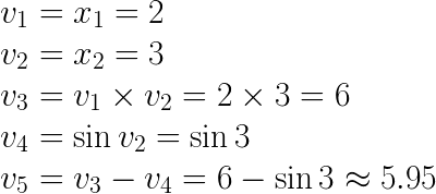
Primal Trace
The primal trace simply stores all the intermediate computations of each node
But our goal is to compute
![]()
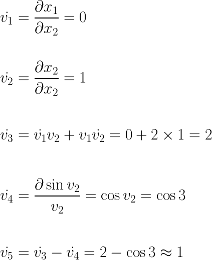
Which we can do via the Dual Trace where we differentiate each expression v with respect to x_2.
Dual Trace
And since we compute v̇_i at the same time as v_i then we can calculate a derivative at the same time as evaluating a function with no memory overhead.
it's not spelled out here, but the trick is to turn x_2 into x_2 + 1e, and then apply dual arithmetics, see from Dual Numbers & Automatic Differentiation « The blog at the bottom of the sea:
Using ε for Automatic Differentiation
You can use dual number operations on numbers to calculate the value of f(x) while also calculating f'(x) at the same time. I’ll show you how with a simple example using addition and multiplication like we went over above.
We’ll start with the function f(x)=3x+2, and calculate f(4) and f'(4).
the first thing we do is convert our 4 into a dual number, using 1 for the dual component, since we are plugging it in for the value of x, which has a derivative of 1.
4+1ε
Next, we want to multiply that by the constant 3, using 0 for the dual component since it is just a constant (and the derivative of a constant is 0)
(4+1ε) * (3 + 0ε) =
12 + 0ε + 3ε + 0ε^2 =
12 + 3eLastly, we need to add the constant 2, using 0 again for the dual component since it’s just a constant.
(12 + 3ε) + (2 + 0ε) =
14 + 3εIn our result, the real number component (14) is the value of f(4) and the dual component (3) is the derivative f'(4), which is correct if you work it out!
Let’s try f(5). First we convert 5 to a dual number, with the dual component being 1.
5 + 1ε
Next we need to multiply it by the constant 3 (which has a dual component of 0)
(5 + 1ε) * (3 + 0e) =
15 + 0ε + 3ε + 0ε^2 =
15 + 3εNow, we add the constant 2 (which has a dual component of 0 again since it’s just a constant)
(15 + 3ε) + (2 + 0ε) =
17 + 3εSo, our answer says that f(5) = 17, and f'(5) = 3, which again you can verify is true!
Quadratic Example
The example above worked well but it was a linear function. What if we want to do a function like f(x) = 5x^2 + 4x + 1?
Let’s calculate f(2). We are going to first calculate the 5x^2 term, so we need to start by making a dual number for the function parameter x:
(2 + 1ε)Next, we need to multiply it by itself to make x^2:
(2 + 1ε) * (2 + 1ε) =
4 + 2ε + 2ε + 1ε^2 =
4 + 4ε(remember that ε^2 is 0, so the last term disappears)
next, we multiply that by the constant 5 to finish making the 5x^2 term:
(4 + 4ε) * (5 + 0ε) =
20 + 0ε + 20ε + 0ε^2 =
20 + 20εNow, putting that number aside for a second we need to calculate the “4x” term by multiplying the value we plugged in for x by the constant 4
(2 + 1ε) * (4 + 0ε) =
8 + 0ε + 4ε + 0ε^2 =
8 + 4εNext, we need to add the last 2 values together (the 5x^2 term and the 4x term):
(20 + 20ε) + (8 + 4ε) =
28 + 24εLastly, we need to add in the last term, the constant 1
(28 + 24ε) + (1 + 0ε) =
29 + 24eThere is our answer! For the equation y = 5x^2 + 4x + 1, f(2) = 29 and f'(2) = 24. Check it, it’s correct (:
That said you may have noticed that we only computed the derivative for x_2, in fact we’d need to repeat this process for each input which on deep learning applications is a non starter given that input data is very often high dimensional.
Working with vector valued functions
More generally we’d like to work with vector valued functions f that can take in multiple inputs and produce multiple outputs.
![]()
So we need a way to represent the derivative of each output y with respect to each input x and the Jacobian matrix helps us do this.
The technique we’ve described so far is called Forward Mode Differentiation.
Forward Mode Differentiation really suffers when n is large because you need to do a prime and dual trace for each input variable x_i. But the algorithm scales for free when you increase the number of outputs m so it’s still good for generative applications that need to generate large sequences from small input data seed.
So as a result we need to learn about a different technique called Reverse Mode Differentiation. Most deep learning workflows have n >> m so Reverse Mode Differentiation is the algorithm of choice for back-propagation in Pytorch, Flux.jl, Tensorflow and other Deep Learning libraries.
Reverse Mode Differentiation
Let’s use the same function f as an example of how this works
![]()
Primal Trace
Nothing changes
Dual Trace
The Dual Trace for Reverse Mode AD is more complex than its forward counterpart but the main trick is the chain rule.
The chain rule is a technique to break apart a derivative we don’t know how to solve into derivatives that we do know how to solve.
Applied to the context of a computational graph we can write the chain rule as.
But the v_k we’ll be picking won’t be arbitrary. In fact v_k would be the parent of v_i in the computational graph. If v_k has more than one parent then we sum up the chain rule over all its parents. This is called the Multi-variable chain rule, you can find a proof here
The above expression has a name and it’s called the adjoint of v_i which we’ll denote as ̅v_i.
Given this definition we can then rewrite the adjoint in terms of the adjoint of its parents.
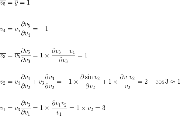
Which gives us a recursive algorithm where we start from the output node y and go back all the way to the input nodes by going over adjoints.
To be clear on what we mean by parent, in the example we’re working with v_3 is a parent of both v_1 and v_2.
The Dual/Adjoint Trace
some typos here and there, but go through the derivation yourself and it should be fairly clear;
note that dual number arithmetic hardly comes to play here, so it's better called adjoint tracing to avoid confusion;
moreover, the adjoints can only be traced after prime trace, unlike forward acc. here prime and dual trace can be executed in sync.
in practice we almost never parallelize tracing, and treat them like sequential steps anyway, so this extra data dependency is counted against the efficiency of reverse acc.
Even though the algorithm was completely different we got back the same result which if you can verify either by symbolic or numeric differentiation.
You can also see how the process is kinda fiddly for a human but is ideally suited for computers.
The amazing thing about Reverse Mode AD is that it computed in one full iteration both of
While the example we worked through with Forward Mode AD only gave us back.
If you’d like to see one more example fully worked out, Step-by-step example of reverse-mode automatic differentiation is another great resource.
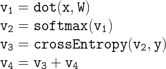
Wengert List for Logistic Regression
And if you want to generalize this idea to deep neural networks you just need to apply either Forward or Reverse Mode AD on a Wengert List that looks something like the below. All of the operations are differentiable and if you’re writing them in a deep learning library, it takes care of making them differentiable for you even if you for e.g have control statements.
But that’s just code? What do you mean it’s a Wengert List? Code that does 1 operation per line is a Wengert List — in languages like Julia this is explicit.
Summary of Forward vs Reverse Mode AD
It’s hard to remember all the mechanics of both algorithms on a first read but you can remember their trade-offs so you know what to use when.
- Forward Mode AD can throw away intermediate results since it’s an iterative algorithm.
- Reverse Mode AD needs to keep all intermediate results in memory since it’s a recursive algorithm.
- Forward Mode AD needs to run once per input to compute the full Jacobian matrix.
- Reverse Mode AD needs to run once per output to compute the full Jacobian matrix.
But it’s also worth remembering that your human time is more valuable than computer storage and deep learning applications mostly have large outputs and small inputs.
Next Steps
Differentiable Programming
This entire discussion may have given you the impression that Automatic Differentiation is a technique for numeric code only. AD is part of a larger programming paradigm called Differentiable Programming where you write your code in a differentiable manner and get its derivative for free. Even control flow operations like for and if admit derivatives.
Within the context of code, a derivative represents a small step forward or backward in the state and the range of applications this opens up is endless.
From Differentiable Physics Engines to Differentiable Ray Tracers to Differentiable Control — I honestly can’t wait to see what the future holds here.
Compilers for Machine Learning
Given a computational graph there’s many tricks you can perform to make it smaller and avoid duplicate data. This is a growing field in of itself as Deep Learning models are memory and compute intensive so any improvements here immediately translate into dollars/bitcoins saved. The effort I’m following the closest is Swift for Tensorflow Graph Program Extraction but I’m sure there are others, since compilers for ML is far from being a solved problem.
If you know of any or are working on compilers for ML please reach out, I’d love to check it out and blog about it!
We programmers don’t use enough math in our work — if we did, we wouldn’t write as much code.


