OpenCV-图像金字塔
图像金字塔
什么是图像金字塔(pyramid),cv.pyrUp(),cv.pyrDown()
概念:
图像金字塔是同一图像的不同分辨率的子图集合,

如何生成图像金字塔:

1,向下取样:
两个步骤:

通过这样做,M×N 图像变成M/2×N/2图像。因此面积减少到原始面积的四分之一。它称为Octave。
2,向上取样:

为何乘4?

通过这样做,M×N M×N图像变成2M×2N 图像。因此面积增大到原始面积的四倍。
注:向下取样和向上取样不是互逆的,
向下取样代码:
import cv2 as cv
if __name__ == '__main__':
    img = cv.imread("images/4.jpg")
    res = cv.pyrDown(img) # 向下取样
    res2 = cv.pyrDown(res) # 向下取样
    res3 = cv.pyrDown(res2) # 向下取样
    cv.imshow("img",img)
    cv.imshow("res",res)
    cv.imshow("res2",res2)
    cv.imshow("res3",res3)

    cv.waitKey(0)
    cv.destroyAllWindows()
向上取样代码:
import cv2 as cv
if __name__ == '__main__':
    img = cv.imread("images/zzz.jpg")
    res = cv.pyrUp(img) # 向上取样
    res2 = cv.pyrUp(res) # 向上取样
    res3 = cv.pyrUp(res2) # 向上取样
    cv.imshow("img",img)
    cv.imshow("res",res)
    cv.imshow("res2",res2)
    cv.imshow("res3",res3)

    cv.waitKey(0)
    cv.destroyAllWindows()
拉普拉斯金字塔
前面的金字塔叫做高斯金字塔,因为使用的是高斯卷积核,
拉普拉斯金字塔是在高斯金字塔基础之上的新的金字塔,

import cv2 as cv

if __name__ == '__main__':
    img = cv.imread("images/lena.jpg")

    down1 = cv.pyrDown(img)
    res = img - cv.pyrUp(down1)

    down2 = cv.pyrDown(down1)
    res2 = down1 - cv.pyrUp(down2)

    cv.imshow("img", img)
    cv.imshow("res", res)
    cv.imshow("res2", res2)

    cv.waitKey(0)
    cv.destroyAllWindows()
使用金字塔进行图像融合
金字塔的一种应用是图像融合。例如,在图像拼接中,您需要将两个图像堆叠在一起,但是由于图像之间的不连续性,可能看起来不太好。在这种情况下,使用金字塔混合图像可以无缝混合,而不会在图像中保留大量数据。一个经典的例子是将两种水果,橙和苹果混合在一起
import cv2 as cv
import numpy as np
import matplotlib.pyplot as plt

if __name__ == '__main__':
    apple = cv.imread('images/apple.jpg')
    orange = cv.imread('images/orange.jpg')
    apple = cv.resize(apple, (320, 320), interpolation=cv.INTER_CUBIC)  # 将原图300,300 调整到64 的整数倍,因为下面有6层金字塔,这样就不会有小数出现
    orange = cv.resize(orange, (320, 320), interpolation=cv.INTER_CUBIC)

    # 生成apple的高斯金字塔
    G = apple.copy()[..., ::-1]
    plt.subplot(3, 3, 1), plt.imshow(G, cmap='gray')
    plt.title('Original'), plt.xticks([]), plt.yticks([])
    gaussianAppleList = [G]
    for i in range(6):
        G = cv.pyrDown(G)
        gaussianAppleList.append(G)
        plt.subplot(3, 3, i + 2), plt.imshow(G, cmap='gray')
        plt.title(f'Gaussian{i + 1}'), plt.xticks([]), plt.yticks([])
    plt.show()
    # 生成orange的高斯金字塔
    G = orange.copy()[..., ::-1]
    plt.subplot(3, 3, 1), plt.imshow(G, cmap='gray')
    plt.title('Original'), plt.xticks([]), plt.yticks([])
    gaussianOrangeList = [G]
    for i in range(6):
        G = cv.pyrDown(G)
        gaussianOrangeList.append(G)
        plt.subplot(3, 3, i + 2), plt.imshow(G, cmap='gray')
        plt.title(f'Gaussian{i + 1}'), plt.xticks([]), plt.yticks([])
    plt.show()
    # 生成apple的拉普拉斯金字塔
    lpApple = [gaussianAppleList[5]]
    for i in range(5, 0, -1):
        gaussianUp = cv.pyrUp(gaussianAppleList[i])
        L = cv.subtract(gaussianAppleList[i - 1], gaussianUp)
        lpApple.append(L)
        plt.subplot(3, 3, 6 - i), plt.imshow(L, cmap='gray')
        plt.title(f'Lp Apple{6 - i}'), plt.xticks([]), plt.yticks([])
    plt.show()
    # 生成B的拉普拉斯金字塔
    lpOrange = [gaussianOrangeList[5]]
    for i in range(5, 0, -1):
        gaussianUp = cv.pyrUp(gaussianOrangeList[i])
        L = cv.subtract(gaussianOrangeList[i - 1], gaussianUp)
        lpOrange.append(L)
        plt.subplot(3, 3, 6 - i), plt.imshow(L, cmap='gray')
        plt.title(f'Lp Orange{6 - i}'), plt.xticks([]), plt.yticks([])
    plt.show()

    # # 在每个拉普拉斯金字塔级别中加入苹果的左半部分和橙子的右半部分
    lpNewList = []
    i = 0
    for lp1, lp2 in zip(lpApple, lpOrange):
        rows, cols, dpt = lp1.shape
        lp_new = np.hstack((lp1[:, 0:cols // 2], lp2[:, cols // 2:]))  # 水平方向 连接
        lpNewList.append(lp_new)
        plt.subplot(3, 3, i + 1), plt.imshow(lp_new, cmap='gray')
        plt.title(f'Lp New {i + 1}'), plt.xticks([]), plt.yticks([])
        i += 1
    plt.show()

    # 重建原始图像
    lp_ = lpNewList[0]  # 最模糊 的 lp
    plt.subplot(3, 3, 1), plt.imshow(lp_, cmap='gray')
    plt.title(f'Lp ReBuilt 1'), plt.xticks([]), plt.yticks([])
    for i in range(1, 6):
        lp_ = cv.pyrUp(lp_)
        lp_ = cv.add(lp_, lpNewList[i])
        plt.subplot(3, 3, i + 1), plt.imshow(lp_, cmap='gray')
        plt.title(f'Lp ReBuilt {i + 1}'), plt.xticks([]), plt.yticks([])
    plt.show()

    # ================================
    # 如果直接将图像 拼接
    cols = apple.shape[1]
    sc = np.hstack((apple[:, :cols // 2, ::-1], orange[:, cols // 2:, ::-1]))
    plt.subplot(1, 2, 1), plt.imshow(sc, cmap='gray')
    plt.title(f'Simply Concat'), plt.xticks([]), plt.yticks([])
    plt.subplot(1, 2, 2), plt.imshow(lp_, cmap='gray')
    plt.title(f'Pyramid Process'), plt.xticks([]), plt.yticks([])
    plt.show()
轮廓
边缘检测虽然能够检测出边缘,但边缘是不连续的,图像轮廓是指将边缘连接起来形成一个整体,
轮廓是什么,如何查找轮廓,绘制轮廓
cv.findContours(),cv.drawContours()
什么是轮廓:
轮廓可以简单地解释为连接具有相同颜色或强度的所有连续点(沿边界)的曲线。轮廓是用于形状分析以及对象检测和识别的有用工具。
1,为了获得更高的准确性,请使用二进制图像。因此,在找到轮廓之前,请应用阈值或canny边缘检测
2,从OpenCV 3.2开始,findContours()不再修改源图像
3,在OpenCV中,找到轮廓就像从黑色背景中找到白色物体。因此请记住,要找到的对象应该是白色,背景应该是黑色
查找轮廓并画出:
findcontour()函数中有三个参数,第一个是源图像,第二个是轮廓检索模式,第三个是轮廓逼近方法。输出等高线和层次结构。轮廓是图像中所有轮廓的Python列表。每个单独的轮廓是一个(x,y)坐标的Numpy数组的边界点的对象。


import cv2 as cv
import numpy as np
import matplotlib.pyplot as plt

if __name__ == '__main__':
    img = cv.imread('images/lena.jpg')
    cv.imshow("img",img)
    imgGray = cv.cvtColor(img,cv.COLOR_BGR2GRAY)
    _, thresh = cv.threshold(imgGray, 127, 255, 0)

    # contours 是个列表,包含了所有的轮廓,每个轮廓是由点组成的
    contours, hierarchy = cv.findContours(thresh, cv.RETR_TREE, cv.CHAIN_APPROX_SIMPLE)  # 第一个是源图像,第二个是轮廓检索模式,第三个是轮廓逼近方法

    # 绘制轮廓 到 原图上
    # cv.drawContours(img,contours,-1,(0,255,0),1) # 绘制所有的轮廓

    # cv.drawContours(img,contours,3,(0,255,0),1) # 绘制第四个轮廓
    # 但是在大多数情况下,以下方法会很有用:
    cnt = contours[3]
    cv.drawContours(img, [cnt], 0, (0, 255, 0), 1)
    cv.imshow("dst",img)

    cv.waitKey(0)
    cv.destroyAllWindows()
轮廓特征:
如何找到轮廓的面积,周长,质心,边界框等
cv.moment() cv.contourArea() cv.arcLenth()
1 特征矩
特征矩可以帮助您计算一些特征,例如物体的质心,物体的面积等。
函数cv.moments()提供了所有计算出的矩值的字典
import cv2 as cv
import numpy as np
import matplotlib.pyplot as plt

if __name__ == '__main__':
    img = cv.imread('images/star.jpg')
    imgGray = cv.cvtColor(img, cv.COLOR_BGR2GRAY)
    _, thresh = cv.threshold(imgGray, 50, 255, 0)
    # cv.imshow("imgGray",imgGray)
    # cv.imshow("thresh",thresh)
    contours, hierarchy = cv.findContours(thresh, cv.RETR_TREE, cv.CHAIN_APPROX_SIMPLE)
    cnt = contours[0]
    M = cv.moments(cnt)
    print(M)
    '''
    {'m00': 29596.0, 'm10': 3305242.5, 'm01': 2100078.833333333, 'm20': 489679620.8333333, 'm11': 236742605.8333333, 'm02': 198434862.5, 'm30': 81469692246.65001, 'm21': 35396123621.833336, 'm12': 22497281737.8, 'm03': 21186929032.75, 'mu20': 120554469.33291936, 'mu11': 2208553.485592097, 'mu02': 49417052.45084831, 'mu30': -143816517.0492096, 'mu21': 156043323.3139515, 'mu12': 22906353.578845024, 'mu03': 93258731.11600876, 'nu20': 0.1376313210231425, 'nu11': 0.0025214007863357023, 'nu02': 0.056417105458760115, 'nu30': -0.0009543907471199464, 'nu21': 0.0010355299027977676, 'nu12': 0.00015201043909599888, 'nu03': 0.0006188807231008864}
    '''

    cv.waitKey(0)
    cv.destroyAllWindows()
质心:
import cv2 as cv
import numpy as np
import matplotlib.pyplot as plt

if __name__ == '__main__':
    img = cv.imread('images/star.jpg')
    imgGray = cv.cvtColor(img, cv.COLOR_BGR2GRAY)
    _, thresh = cv.threshold(imgGray, 50, 255, 0)
    # cv.imshow("imgGray",imgGray)
    # cv.imshow("thresh",thresh)
    contours, hierarchy = cv.findContours(thresh, cv.RETR_TREE, cv.CHAIN_APPROX_SIMPLE)
    cnt = contours[0]
    M = cv.moments(cnt)
    # print(M)
    cx = int(M['m10'] / M['m00'])
    cy = int(M['m01'] / M['m00'])
    print(cx,cy)
2 轮廓面积
轮廓区域由函数cv.contourArea()或从矩M['m00']中给出。
import cv2 as cv
import numpy as np
import matplotlib.pyplot as plt

if __name__ == '__main__':
    img = cv.imread('images/star.jpg')
    imgGray = cv.cvtColor(img, cv.COLOR_BGR2GRAY)
    _, thresh = cv.threshold(imgGray, 50, 255, 0)
    # cv.imshow("imgGray",imgGray)
    # cv.imshow("thresh",thresh)
    contours, hierarchy = cv.findContours(thresh, cv.RETR_TREE, cv.CHAIN_APPROX_SIMPLE)
    cnt = contours[0]
    M = cv.moments(cnt)
    # print(M)
    # 面积
    print(M['m00'])
import cv2 as cv
import numpy as np
import matplotlib.pyplot as plt
if __name__ == '__main__':
img = cv.imread('images/star.jpg')
imgGray = cv.cvtColor(img, cv.COLOR_BGR2GRAY)
_, thresh = cv.threshold(imgGray, 50, 255, 0)
# cv.imshow("imgGray",imgGray)
# cv.imshow("thresh",thresh)
contours, hierarchy = cv.findContours(thresh, cv.RETR_TREE, cv.CHAIN_APPROX_SIMPLE)
cnt = contours[0]
# 面积
# M = cv.moments(cnt)
# print(M)
# print(M['m00'])
print(cv.contourArea(cnt))3 轮廓周长
也称为弧长。可以使用cv.arcLength()函数找到它。第二个参数指定形状是闭合轮廓(True)还是曲线
import cv2 as cv
import numpy as np
import matplotlib.pyplot as plt

if __name__ == '__main__':
    img = cv.imread('images/star.jpg')
    imgGray = cv.cvtColor(img, cv.COLOR_BGR2GRAY)
    _, thresh = cv.threshold(imgGray, 50, 255, 0)
    # cv.imshow("imgGray",imgGray)
    # cv.imshow("thresh",thresh)
    contours, hierarchy = cv.findContours(thresh, cv.RETR_TREE, cv.CHAIN_APPROX_SIMPLE)
    cnt = contours[0]
    # 周长
    perimeter = cv.arcLength(cnt, True)
    print(perimeter)
4 轮廓近似
根据我们指定的精度,它可以将轮廓形状近似为顶点数量较少的其他形状。它是Douglas-Peucker算法的实现。
第二个参数称为epsilon,它是从轮廓到近似轮廓的最大距离。
import cv2 as cv
import numpy as np
import matplotlib.pyplot as plt

if __name__ == '__main__':
    img = cv.imread('images/star.jpg')
    imgGray = cv.cvtColor(img, cv.COLOR_BGR2GRAY)
    _, thresh = cv.threshold(imgGray, 50, 255, 0)
    # cv.imshow("imgGray",imgGray)
    # cv.imshow("thresh",thresh)
    contours, hierarchy = cv.findContours(thresh, cv.RETR_TREE, cv.CHAIN_APPROX_SIMPLE)
    cnt = contours[0]

    dst = cv.drawContours(img, [cnt], 0, (0, 255, 0), 1)
    cv.imshow("dst", dst)

    # 轮廓近似
    epsilon = 0.1 * cv.arcLength(cnt, True)
    approx = cv.approxPolyDP(cnt, epsilon, True)
    # print(approx) # 将近似曲线的点 画在图上 用蓝色标出
    res1 = cv.polylines(img, [approx], True, (255, 0, 0))
    cv.imshow("res1",res1)

    # 改变epsilon
    epsilon = 0.01 * cv.arcLength(cnt, True)
    approx = cv.approxPolyDP(cnt, epsilon, True)
    res2 = cv.polylines(img, [approx], True, (255, 0, 0))
    cv.imshow("res2",res2)


    cv.waitKey(0)
    cv.destroyAllWindows()
在第二张图片中,蓝线显示了ε=弧长的10%时的近似曲线。第三幅图显示了ε=弧长度的1%时的情况。

5 轮廓凸包
凸包外观看起来与轮廓逼近相似,但不相似(在某些情况下两者可能提供相同的结果)。在这里,cv.convexHull()函数检查曲线是否存在凸凹缺陷并对其进行校正。一般而言,凸曲线是始终凸出或至少平坦的曲线。如果在内部凸出,则称为凸度缺陷。例如,检查下面的手的图像。红线显示手的凸包。双向箭头标记显示凸度缺陷,这是凸包与轮廓线之间的局部最大偏差
import cv2 as cv
import numpy as np
import matplotlib.pyplot as plt

if __name__ == '__main__':
    img = cv.imread('images/hand.jpg')
    imgGray = cv.cvtColor(img, cv.COLOR_BGR2GRAY)
    _, thresh = cv.threshold(imgGray, 50, 255, 0)

    contours, hierarchy = cv.findContours(thresh, cv.RETR_TREE, cv.CHAIN_APPROX_SIMPLE)
    cnt = contours[0]
    hull = cv.convexHull(cnt) # cv.convexHull()函数检查曲线是否存在凸凹缺陷并对其进行校正

    res1 = cv.polylines(img, [hull], True, (255, 0, 0))
    cv.imshow("res1", res1)

    dst = cv.drawContours(img, [cnt], 0, (0, 255, 0), 1)
    cv.imshow("dst", dst)

    cv.waitKey(0)
    cv.destroyAllWindows()
6 检查凸度
cv.isContourConvex()具有检查曲线是否凸出的功能。它只是返回True还是False
ret = cv.isContourConvex(cnt)
7 边界矩形
a, 直角矩形
它不考虑物体的旋转。所以边界矩形的面积不是最小的。它是由函数cv.boundingRect()找到的。
import cv2 as cv
import numpy as np
import matplotlib.pyplot as plt

if __name__ == '__main__':
    img = cv.imread('images/aaa.jpg')
    imgGray = cv.cvtColor(img, cv.COLOR_BGR2GRAY)
    _, thresh = cv.threshold(imgGray, 50, 255, 0)

    contours, hierarchy = cv.findContours(thresh, cv.RETR_TREE, cv.CHAIN_APPROX_SIMPLE)
    cnt = contours[0]

    x,y,w,h = cv.boundingRect(cnt)
    cv.rectangle(img,(x,y),(x+w,y+h),(255,0,0),2)

    dst = cv.drawContours(img, [cnt], 0, (0, 255, 0), 1)
    cv.imshow("dst", dst)

    cv.waitKey(0)
    cv.destroyAllWindows()
b, 旋转矩形
边界矩形是用最小面积绘制的,所以它也考虑了旋转。使用的函数是cv.minAreaRect()。它返回一个Box2D结构,其中包含以下细节 -(中心(x,y),(宽度,高度),旋转角度)。但要画出这个矩形,我们需要矩形的四个角。它由函数cv.boxPoints()获得
import cv2 as cv
import numpy as np
import matplotlib.pyplot as plt

if __name__ == '__main__':
    img = cv.imread('images/aaa.jpg')
    imgGray = cv.cvtColor(img, cv.COLOR_BGR2GRAY)
    _, thresh = cv.threshold(imgGray, 50, 255, 0)

    contours, hierarchy = cv.findContours(thresh, cv.RETR_TREE, cv.CHAIN_APPROX_SIMPLE)
    cnt = contours[0]

    rect = cv.minAreaRect(cnt)
    box = np.int0(cv.boxPoints(rect)).reshape(-1,1,2)
    cv.polylines(img,[box],True,(0,0,255),2)

    dst = cv.drawContours(img, [cnt], 0, (0, 255, 0), 1)
    cv.imshow("dst", dst)

    cv.waitKey(0)
    cv.destroyAllWindows()
8 最小闭合圆
使用函数cv.minEnclosingCircle()查找对象的圆周。它是一个以最小面积完全覆盖物体的圆
import cv2 as cv
import numpy as np
import matplotlib.pyplot as plt

if __name__ == '__main__':
    img = cv.imread('images/aaa.jpg')
    imgGray = cv.cvtColor(img, cv.COLOR_BGR2GRAY)
    _, thresh = cv.threshold(imgGray, 50, 255, 0)

    contours, hierarchy = cv.findContours(thresh, cv.RETR_TREE, cv.CHAIN_APPROX_SIMPLE)
    cnt = contours[0]

    (x, y), radius = cv.minEnclosingCircle(cnt)
    center = (int(x), int(y))
    radius = int(radius)
    cv.circle(img, center, radius, (255, 0, 0), 2)

    dst = cv.drawContours(img, [cnt], 0, (0, 255, 0), 1)
    cv.imshow("dst", dst)

    cv.waitKey(0)
    cv.destroyAllWindows()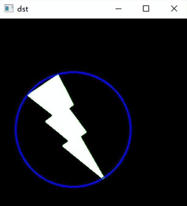
9 拟合一个椭圆
import cv2 as cv
import numpy as np
import matplotlib.pyplot as plt

if __name__ == '__main__':
    img = cv.imread('images/aaa.jpg')
    imgGray = cv.cvtColor(img, cv.COLOR_BGR2GRAY)
    _, thresh = cv.threshold(imgGray, 50, 255, 0)

    contours, hierarchy = cv.findContours(thresh, cv.RETR_TREE, cv.CHAIN_APPROX_SIMPLE)
    cnt = contours[0]

    ellipse = cv.fitEllipse(cnt)
    cv.ellipse(img, ellipse, (255, 0, 0), 2)

    dst = cv.drawContours(img, [cnt], 0, (0, 255, 0), 1)
    cv.imshow("dst", dst)

    cv.waitKey(0)
    cv.destroyAllWindows()
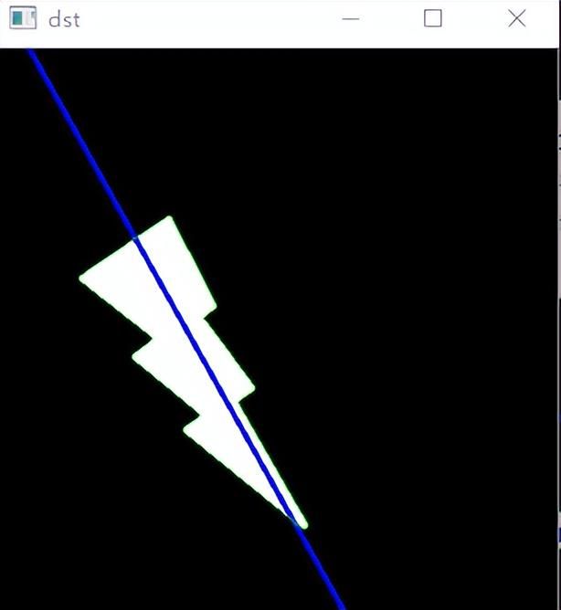
9 拟合直线
import cv2 as cv
import numpy as np
import matplotlib.pyplot as plt

if __name__ == '__main__':
    img = cv.imread('images/aaa.jpg')
    imgGray = cv.cvtColor(img, cv.COLOR_BGR2GRAY)
    _, thresh = cv.threshold(imgGray, 50, 255, 0)

    contours, hierarchy = cv.findContours(thresh, cv.RETR_TREE, cv.CHAIN_APPROX_SIMPLE)
    cnt = contours[0]

    rows, cols = img.shape[:2]
    [vx, vy, x, y] = cv.fitLine(cnt, cv.DIST_L2, 0, 0.01, 0.01)
    lefty = int((-x * vy / vx) + y)
    righty = int(((cols - x) * vy / vx) + y)
    cv.line(img, (cols - 1, righty), (0, lefty), (255, 0, 0), 2)

    dst = cv.drawContours(img, [cnt], 0, (0, 255, 0), 1)
    cv.imshow("dst", dst)

    cv.waitKey(0)
    cv.destroyAllWindows()