基于随机森林的otto商品分类

数据集介绍

Otto Group数据集来源于《Otto Group Product Classification Challenge》。Otto集团是世界上最大的电子商务公司之一，在20多个国家拥有子公司。我们每天在全球销售数百万种产品，在我们的产品线中添加了数千种产品。

我们公司对我们产品性能的一致性分析至关重要。然而，由于我们的全球基础设施不同，许多相同的产品被分类不同。因此，我们的产品分析的质量在很大程度上取决于对类似产品进行准确分类的能力。分类越好，我们对产品范围的了解就越多。

在这次竞争中，我们为超过200000种产品提供了一个具有93项功能的数据集。目的是建立一个预测模型，能够区分我们的主要产品类别。获奖模型将采用开源模式。

奥托集团产品分类数据集：

• Target：共9个商品类别
• Features：93个特征：整数型特征

import pandas as pd
import numpy as np
import os
import matplotlib.pyplot as plt
import seaborn as sns
from sklearn.preprocessing import LabelEncoder, OneHotEncoder
from sklearn.metrics import log_loss
from sklearn.model_selection import GridSearchCV
%matplotlib inline

读取数据

查看当前工作路径

os.path.abspath('.')

读取数据

data = pd.read_csv("./otto-group-product-classification-challenge/train.csv")
data.head()

	id	feat_1	feat_2	feat_3	feat_4	feat_5	feat_6	feat_7	feat_8	feat_9	...	feat_85	feat_86	feat_87	feat_88	feat_89	feat_90	feat_91	feat_92	feat_93	target
0	1	1	0	0	0	0	0	0	0	0	...	1	0	0	0	0	0	0	0	0	Class_1
1	2	0	0	0	0	0	0	0	1	0	...	0	0	0	0	0	0	0	0	0	Class_1
2	3	0	0	0	0	0	0	0	1	0	...	0	0	0	0	0	0	0	0	0	Class_1
3	4	1	0	0	1	6	1	5	0	0	...	0	1	2	0	0	0	0	0	0	Class_1
4	5	0	0	0	0	0	0	0	0	0	...	1	0	0	0	0	1	0	0	0	Class_1

5 rows × 95 columns

# 数据维度
data.shape

(61878, 95)

数据特征分析

# 描述性统计
data.describe()

	id	feat_1	feat_2	feat_3	feat_4	feat_5	feat_6	feat_7	feat_8	feat_9	...	feat_84	feat_85	feat_86	feat_87	feat_88	feat_89	feat_90	feat_91	feat_92	feat_93
count	61878.000000	61878.00000	61878.000000	61878.000000	61878.000000	61878.000000	61878.000000	61878.000000	61878.000000	61878.000000	...	61878.000000	61878.000000	61878.000000	61878.000000	61878.000000	61878.000000	61878.000000	61878.000000	61878.000000	61878.000000
mean	30939.500000	0.38668	0.263066	0.901467	0.779081	0.071043	0.025696	0.193704	0.662433	1.011296	...	0.070752	0.532306	1.128576	0.393549	0.874915	0.457772	0.812421	0.264941	0.380119	0.126135
std	17862.784315	1.52533	1.252073	2.934818	2.788005	0.438902	0.215333	1.030102	2.255770	3.474822	...	1.151460	1.900438	2.681554	1.575455	2.115466	1.527385	4.597804	2.045646	0.982385	1.201720
min	1.000000	0.00000	0.000000	0.000000	0.000000	0.000000	0.000000	0.000000	0.000000	0.000000	...	0.000000	0.000000	0.000000	0.000000	0.000000	0.000000	0.000000	0.000000	0.000000	0.000000
25%	15470.250000	0.00000	0.000000	0.000000	0.000000	0.000000	0.000000	0.000000	0.000000	0.000000	...	0.000000	0.000000	0.000000	0.000000	0.000000	0.000000	0.000000	0.000000	0.000000	0.000000
50%	30939.500000	0.00000	0.000000	0.000000	0.000000	0.000000	0.000000	0.000000	0.000000	0.000000	...	0.000000	0.000000	0.000000	0.000000	0.000000	0.000000	0.000000	0.000000	0.000000	0.000000
75%	46408.750000	0.00000	0.000000	0.000000	0.000000	0.000000	0.000000	0.000000	1.000000	0.000000	...	0.000000	0.000000	1.000000	0.000000	1.000000	0.000000	0.000000	0.000000	0.000000	0.000000
max	61878.000000	61.00000	51.000000	64.000000	70.000000	19.000000	10.000000	38.000000	76.000000	43.000000	...	76.000000	55.000000	65.000000	67.000000	30.000000	61.000000	130.000000	52.000000	19.000000	87.000000

8 rows × 94 columns

# 查看数据分布
sns.countplot(x=data.target)

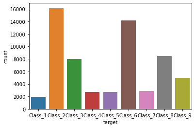
可以看出，数据类别不均衡

数据处理

# 特征值
x = data.drop(["id","target"], axis=1)
# 目标值
y = data["target"]

x.head()

	feat_1	feat_2	feat_3	feat_4	feat_5	feat_6	feat_7	feat_8	feat_9	feat_10	...	feat_84	feat_85	feat_86	feat_87	feat_88	feat_89	feat_90	feat_91	feat_92	feat_93
0	1	0	0	0	0	0	0	0	0	0	...	0	1	0	0	0	0	0	0	0	0
1	0	0	0	0	0	0	0	1	0	0	...	0	0	0	0	0	0	0	0	0	0
2	0	0	0	0	0	0	0	1	0	0	...	0	0	0	0	0	0	0	0	0	0
3	1	0	0	1	6	1	5	0	0	1	...	22	0	1	2	0	0	0	0	0	0
4	0	0	0	0	0	0	0	0	0	0	...	0	1	0	0	0	0	1	0	0	0

5 rows × 93 columns

y.value_counts().sort_index()

# 由于数据集较大，同时样本类别分布不均衡，故通过欠采样缩小数据集规模
# from imblearn.under_sampling import RandomUnderSampler

把标签值转换为数字

y = LabelEncoder().fit_transform(y)
y

array([0, 0, 0, ..., 8, 8, 8])

分割数据

from sklearn.model_selection import train_test_split

x_train, x_test, y_train, y_test = train_test_split(x,y, test_size=0.2)
x_train.shape, y_train.shape, y_test.shape, x_test.shape

((49502, 93), (49502,), (12376,), (12376, 93))

模型训练

from sklearn.ensemble import RandomForestClassifier
rf_model = RandomForestClassifier(oob_score=True)
rf_model.fit(x_train, y_train)

RandomForestClassifier(oob_score=True)

y_pred = rf_model.predict(x_test)

模型评估

# 模型在训练集上的准确率 
rf_model.score(x_train, y_train)

0.9999797987960083

# 模型在测试集上的准确率 
rf_model.score(x_test, y_test)

0.8089043309631545

# 包外估计
rf_model.oob_score_

0.7993818431578522

encoder = OneHotEncoder(sparse=False)
y_test = encoder.fit_transform(y_test.reshape(-1,1))
y_pred = encoder.fit_transform(y_pred.reshape(-1,1))
y_test,

(array([[0., 0., 1., ..., 0., 0., 0.],
        [0., 1., 0., ..., 0., 0., 0.],
        [0., 0., 0., ..., 1., 0., 0.],
        ...,
        [0., 0., 0., ..., 0., 0., 1.],
        [0., 0., 1., ..., 0., 0., 0.],
        [1., 0., 0., ..., 0., 0., 0.]]),)

 y_pred

array([[0., 0., 1., ..., 0., 0., 0.],
       [0., 1., 0., ..., 0., 0., 0.],
       [0., 0., 0., ..., 0., 1., 0.],
       ...,
       [0., 0., 0., ..., 0., 0., 1.],
       [0., 1., 0., ..., 0., 0., 0.],
       [0., 0., 0., ..., 0., 0., 0.]])

# logloss评估
log_loss(y_test, y_pred, eps=1e-15, normalize=True)

6.600210582899472

# 以概率形式输出
y_pred_proba = rf_model.predict_proba(x_test)
y_pred_proba

array([[0.  , 0.2 , 0.77, ..., 0.  , 0.02, 0.  ],
       [0.02, 0.48, 0.16, ..., 0.06, 0.  , 0.  ],
       [0.03, 0.02, 0.03, ..., 0.3 , 0.32, 0.02],
       ...,
       [0.12, 0.01, 0.05, ..., 0.08, 0.11, 0.53],
       [0.01, 0.56, 0.32, ..., 0.01, 0.02, 0.  ],
       [0.18, 0.09, 0.01, ..., 0.1 , 0.2 , 0.14]])

rf_model.oob_score_

0.7993818431578522

log_loss(y_test, y_pred_proba, eps=1e-15, normalize=True)

0.6232249914857839