R语言绘制堆叠面积图

areaplot包绘制堆叠面积图

library(areaplot)
#数据
df <- longley
x <- df$Year
y <- df[, c(1, 2, 3, 4, 6, 8)]
# 颜色
cols <- hcl.colors(6, palette = "viridis", alpha = 0.8)

#绘图
areaplot(x, y, prop = TRUE, col = cols,
         border = "white",
         lwd = 1,
         lty = 1)

#添加图例标签
areaplot(x, y, prop = TRUE, col = cols,
         legend = TRUE,
         args.legend = list(x = "topleft", cex = 0.65,
                            bg = "white", bty = "o"))

ggplot2绘制堆叠面积图

library(reshape2)
library(ggplot2)

#读取数据
phylum <- read.delim('otu2.txt', row.names = 1, sep = '\t', stringsAsFactors = FALSE, check.names = FALSE)

#求和、排序
phylum$sum <- rowSums(phylum)
phylum <- phylum[order(phylum$sum, decreasing = TRUE), ]

#选取 top10，将其他的合并为“Others”
phylum_top10 <- phylum[1:10, -ncol(phylum)]
phylum_top10['Others', ] <- 1 - colSums(phylum_top10)

#输出文件
write.csv(phylum_top10, 'phylum_top10.csv', quote = FALSE)

#表格样式重排
phylum_top10$Taxonomy <- factor(rownames(phylum_top10), levels = rev(rownames(phylum_top10)))
phylum_top10 <- melt(phylum_top10, id = 'Taxonomy')
names(phylum_top10)[2] <- 'sample'

#合并分组信息
group <- read.delim('group2.txt', sep = '\t', stringsAsFactors = FALSE, check.names = FALSE)
phylum_top10 <- merge(phylum_top10, group, by = 'sample', all.x = TRUE)

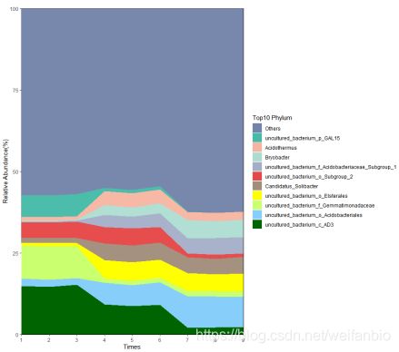
##绘图
p <- ggplot(phylum_top10, aes(x = times, y = 100 * value, fill = Taxonomy)) +
  geom_area() +
  labs(x = 'Times', y = 'Relative Abundance(%)', title = '', fill = 'Top10 Phylum')+ 
  scale_fill_manual(values = c('#3C5488B2', '#00A087B2', '#F39B7FB2', '#91D1C2B2', '#8491B4B2', '#DC0000B2', '#7E6148B2', 'yellow', 'darkolivegreen1', 'lightskyblue', 'darkgreen')) +	#设置颜色
  theme(panel.grid = element_blank(), panel.background = element_rect(color = 'black', fill = 'transparent')) +	#调整背景
  scale_x_continuous(breaks = 1:15, labels = as.character(1:15), expand = c(0, 0)) +	#调整坐标轴轴刻度
  scale_y_continuous(expand = c(0, 0))
p

“作图帮”微信公众号免费分享绘图代码与示例数据。

图图即将推出永久免费的云绘图工具，感兴趣的小伙伴可以关注公众号扫码进群~