python28种极坐标绘图函数总结

python35种绘图函数总结，3D、统计、流场，实用性拉满

matplotlib中的画图函数，大部分情况下只要声明坐标映射是polar，就都可以画出对应的极坐标图。但极坐标和直角坐标的坐标区间不同，所以有些数据和函数关系适合在直角坐标系中展示，而有些则适合在及坐标中展示。

基础图

函数	坐标参数	图形类别
plot	x,y	曲线图
stackplot	x,y	散点图
stem	x,y	茎叶图
scatter	x,y	散点图
polar	x,y	极坐标图
step	x,y	步阶图
bar	x,y	条形图
barh	x,y	横向条形图

bar和barh的对偶关系稍微有些抽象，可以理解为前者是以角度方向为x轴；而barh则是以半径方向为x轴。

代码如下

import matplotlib.pyplot as plt
import numpy as np

x = np.arange(20)/2
y = x

fDct = {"plot" : plt.plot,  "stackplot": plt.stackplot,
        "stem" : plt.stem,  "scatter"  : plt.scatter,         
        "polar": plt.polar, "step"     : plt.step, 
        "bar"  : plt.bar,   "barh"     : plt.barh, }

fig = plt.figure(figsize=(14,6))
for i,key in enumerate(fDct, 1):
    ax = fig.add_subplot(2,4,i, projection="polar")
    fDct[key](x, y)
    plt.title(key)

plt.tight_layout()
plt.show()

误差线

函数	坐标	图形类别
errorbar	x,y,xerr,yerr	误差线
fill_between	x,y1,y2	纵向区间图
fill_betweenx	y, x1, x2	横向区间图

代码如下

x = np.arange(20)/2
y = x
y1, y2 = 0.9*y, 1.1*y
x1, x2 = 0.9*x, 1.1*x
xerr = np.abs([x1, x2])/10
yerr = np.abs([y1, y2])/10

fig = plt.figure(figsize=(12,4))

ax = fig.add_subplot(141, projection='polar')
ax.errorbar(x, y, yerr=yerr)
plt.title("errorbar with yerr")

ax = fig.add_subplot(142, projection='polar')
ax.errorbar(x, y, xerr=xerr)
plt.title("errorbar with xerr")

ax = fig.add_subplot(143, projection='polar')
ax.fill_between(x, y1, y2)
plt.title("fill_between")

ax = fig.add_subplot(144, projection='polar')
ax.fill_betweenx(y, x1, x2)
plt.title("fill_betweenx")

plt.tight_layout()
plt.show()

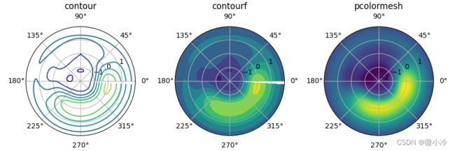
等高线polar

绘图函数	坐标	说明
contour	[x,y,]z	等高线
contourf	[x,y,]z	填充等高线
pcolormesh	[x,y,]z	伪彩图

由于imshow默认其绘图坐标是标准的1x1网格，而在极坐标种，这种网格的尺寸会随着r的增大而增大，从而变得极其不实用，所以下面对极坐标图的演示，就不包含imshow了。

代码如下

X, Y = np.indices([100,100])
X = X/100*np.pi*2
Y = Y/25 - 2
Z = (1 - np.sin(X) + np.cos(X)**5 + Y**3) * np.exp(-Y**2)

fDct = {"contour": plt.contour, "contourf":plt.contourf, 
    "pcolormesh" : plt.pcolormesh}

fig = plt.figure(figsize=(9,3))
for i,key in enumerate(fDct, 1):
    ax = fig.add_subplot(1,3,i, projection='polar')
    fDct[key](X,Y,Z)
    plt.title(key)

plt.tight_layout()
plt.show()

场图polar

绘图函数	坐标	说明
quiver	x,y,u,v	向量场图
streamplot	x,y,u,v	流场图
barbs	x,y,u,v	风场图

代码如下

Y, X = np.indices([10,10])
X = X/10*np.pi*2.5
Y = Y

#Y, X = np.indices([6,6])/0.75 - 4
U = 6*np.sin(X) + Y
V = Y - 6*np.sin(X)

dct = {"quiver":plt.quiver, "streamplot":plt.streamplot, 
       "barbs" :plt.barbs}

fig = plt.figure(figsize=(12,4))

for i,key in enumerate(dct, 1):
    ax = fig.add_subplot(1,3,i,projection='polar')
    dct[key](X,Y,U,V)
    plt.title(key)

plt.tight_layout()
plt.show()

统计图

绘图函数	坐标	说明
hist	x	数据直方图
boxplot	x	箱线图
violinplot	x	小提琴图
enventplot	x	平行线疏密图
hist2d	x,y	二维直方图
hexbin	x,y	钻石图
pie	x	饼图

极坐标在绘制直方图的时候，需要注意其横坐标是以$2\pi$为周期的，也就是说随机变量的最大值和最小值不得相差$2\pi$，否则会导致重叠。

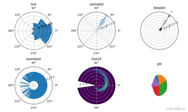
由于极坐标绘图本质上是一种坐标映射，所以并不会把0和360°真正地等同起来，所以在hist2d中，整个图像并没有闭合。而最有意思的是饼图，直接给压扁了，让人很难一下子看出不同组分的比例关系。

代码如下

x = np.random.standard_normal(size=1000)

dct = {"hist"  : plt.hist, "violinplot" : plt.violinplot,
      "boxplot": plt.boxplot}

fig = plt.figure(figsize=(10,6))
for i,key in enumerate(dct, 1):
    ax = fig.add_subplot(2,3,i, projection='polar')
    dct[key](x)
    plt.title(key)

ax = fig.add_subplot(234, projection='polar')
ax.eventplot(x)
plt.title("eventplot")

x = np.random.randn(5000)
y = 1.2 * x + np.random.randn(5000) / 3
ax = fig.add_subplot(235, projection='polar')
ax.hist2d(x, y, bins=[np.arange(-3,3,0.1)] * 2)
plt.title("hist2d")

ax = fig.add_subplot(236, projection='polar')
ax.pie([1,2,3,4,5])
plt.title("pie")

plt.tight_layout()
plt.show()

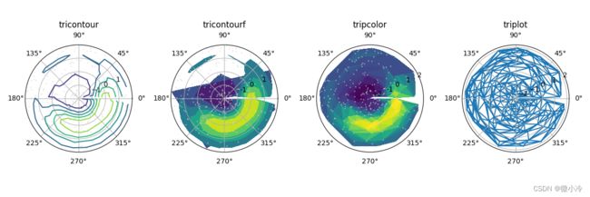
非结构坐标图

绘图函数	坐标	说明
tricontour	x,y,z	非结构等高线
tricontourf	x,y,z	非结构化填充等高线
tricolor	x,y,z	非结构化伪彩图
triplot	x,y	三角连线图

代码如下

x = np.random.uniform(0, np.pi*2, 256)
y = np.random.uniform(-2, 2, 256)
z = (1 - np.sin(x) + np.cos(x)**5 + y**3) * np.exp(-y**2)

levels = np.linspace(z.min(), z.max(), 7)

fig = plt.figure(figsize=(12,4))

ax = fig.add_subplot(141, projection='polar')
ax.plot(x, y, 'o', markersize=1, color='lightgrey', alpha=0.5)
ax.tricontour(x, y, z, levels=levels)
plt.title("tricontour")

ax = fig.add_subplot(142, projection='polar')
ax.plot(x, y, 'o', markersize=1, color='lightgrey', alpha=0.5)
ax.tricontourf(x, y, z, levels=levels)
plt.title("tricontourf")

ax = fig.add_subplot(143, projection='polar')
ax.plot(x, y, 'o', markersize=1, color='lightgrey', alpha=0.5)
ax.tripcolor(x, y, z)
plt.title("tripcolor")

ax = fig.add_subplot(144, projection='polar')
ax.triplot(x,y)
plt.title("triplot")

plt.tight_layout()
plt.show()