深度学习实战（2）用Pytorch搭建双向LSTM

应最近的课程实验要求，要做LSTM和GRU的实验效果对比。LSTM的使用和GRU十分相似，欢迎参考我的另外一篇介绍搭建双向GRU的Blog:https://blog.csdn.net/icestorm_rain/article/details/108395515

参考Pytorch介绍LSTM的官方文档：
其中其定义层时的参数声明方法与GRU完全一致：

所以，我定义LSTM使用以下代码：

torch.nn.LSTM(out_channels, hidden_size, n_layers, batch_first=True,bidirectional=self.bidirectional)

最关键的地方来了，那就是LSTM在做forward计算时要求输入的参数列表和GRU是不一样的！
在官方文档中GRU的输入格式如下：
它只需要 Input以及所有GRU单元的初始隐藏层状态

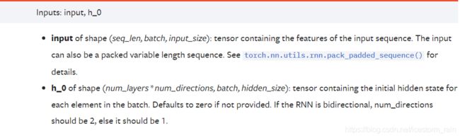
但是对于LSTM来说，还需要所有cell的初始状态，与初始隐藏层状态构成一个二元组进行输入，这是因为LSTM这个神经网络结构的参数是比GRU要多的，具体的可以去学习下两者架构的区别，在此就不做具体介绍了。LSTM的输入格式如下：

所以，我们来看看GRU与LSTM做forward时的代码区别：

# LSTM
output, (hidden, cell_state) = self.lstm(pooled,(hidden,hidden))
# GRU
output, hidden = self.gru(word_inputs, hidden)

其实区别就是在输入输出LSTM比GRU多了一个cell state。
总结到此结束，给个完整的神经网络代码供大家参考，这是一个CNN与LSTM结合的神经网络。

class HomorNetv3(torch.nn.Module):
    def __init__(self, input_dim,hidden_size, out_size, n_layers=1, batch_size=1,window_size=3,out_channels=200,bidirectional=True):
      super(HomorNetv3, self).__init__()

      self.batch_size = batch_size
      self.hidden_size = hidden_size
      self.n_layers = n_layers
      self.out_size = out_size
      self.out_channels = out_channels
      self.bidirectional = bidirectional
      # convolute the word_vectors first
      self.conv = nn.Conv2d(in_channels=1, out_channels=out_channels,kernel_size=(window_size, input_dim))
      self.conv2 = nn.Conv2d(in_channels=1, out_channels=out_channels,kernel_size=(20, input_dim))
      # 这里指定了 BATCH FIRST
      # then put it into GRU layers
      self.lstm = torch.nn.LSTM(out_channels, hidden_size, n_layers, batch_first=True,bidirectional=self.bidirectional)

      # 加了一个线性层，全连接
      if self.bidirectional:
        self.fc1 = torch.nn.Linear(hidden_size*2, 200)
      else:
        self.fc1 = torch.nn.Linear(hidden_size, 200)
      
      # output_layer
      self.fc2 = torch.nn.Linear(200, out_size)
        
    def forward(self, word_inputs, hidden):
       # hidden 就是上下文输出，output 就是 RNN 输出
      #print("word_inputs",word_inputs.shape)
      embedded = word_inputs.unsqueeze(1)
      feature_maps1 = self.conv(embedded)
      feature_maps2 = self.conv2(embedded)
      feature_maps = torch.cat((feature_maps1,feature_maps2),2)
      pooled = self.pool_normalize_function(feature_maps)
      #print("pooled",pooled)
      output, (hidden, cell_state) = self.lstm(pooled,(hidden,hidden))
      #print("gruoutput",output.shape)
      output = self.fc1(output)
      output = self.fc2(output)

      # 仅仅获取 time seq 维度中的最后一个向量
      # the last of time_seq
      output = output[:,-1,:]
      #print("beforesoftmax",output.shape)
      output = F.softmax(output,dim=1)
      print("output",output)
      return output, hidden

    def init_hidden(self):
      # 这个函数写在这里，有一定迷惑性，这个不是模型的一部分，是每次第一个向量没有上下文，在这里捞一个上下文，仅此而已。
      if self.bidirectional:
        hidden = torch.autograd.Variable(torch.zeros(2*self.n_layers, self.batch_size, self.hidden_size, device='cuda'))
      else:
        hidden = torch.autograd.Variable(torch.zeros(self.n_layers, self.batch_size, self.hidden_size, device='cuda'))
      return hidden

    def pool_normalize_function(self,feature_maps):
      ''' pool the vector '''
      feature_maps = feature_maps.squeeze(3)
      # Apply ReLU
      feature_maps = F.relu(feature_maps)
      # Apply the max pooling layer
      pooled = F.max_pool1d(feature_maps, 2)
      pooled = pooled.permute(0,2,1) # 转置矩阵
      normalized = F.normalize(pooled,p=2,dim=2)
      #normalized = normalized.unsqueeze(2)
      return normalized