pyspark MLlib基本使用

MLib

基本概念

• MLib其实就是将数据以RDD的形式进行表示，在分布式数据集上调用各种算法。

使用方法

• MLlib中包含能够在集群上运行良好的并行算法，如kmeans、分布式RF、交替最小二乘等，这能够让MLib中的每个算法都能够适用于大规模数据集
• 也可以将同一算法的不同参数列表通过parallelize()，在不同节点上运行，最终找到性能最好的一组参数，这可以节省小规模数据集上参数选择的时间。

对垃圾邮件进行分类

• 使用基于SGD的LR完成分类任务

from pyspark.mllib.regression import LabeledPoint
from pyspark.mllib.feature import HashingTF
from pyspark.mllib.classification import LogisticRegressionWithSGD

spamFp = "file:///home/hadoop/code/spark/files/spam.txt"
normalFp = "file:///home/hadoop/code/spark/files/normal.txt"
spam= sc.textFile(spamFp)
normal= sc.textFile(normalFp)

# 将每个单词作为一个单独的特征
tf = HashingTF(numFeatures=10000)
spamFeatures = spam.map( lambda email : tf.transform(email.split(" ")) )
normalFeatures = normal.map( lambda email : tf.transform(email.split(" ")) )

# 构建LabelPoint，即每个向量都有它的label，之后联合构成整个训练集
positiveExamples = spamFeatures.map( lambda features : LabeledPoint(1, features) )
negativeExamples = normalFeatures.map( lambda features : LabeledPoint(0, features) )
trainingData = positiveExamples.union(negativeExamples  )
# SGD是迭代算法，因此在这里缓存数据集，加快运行速度
trainingData.cache()

# 训练
model = LogisticRegressionWithSGD.train( trainingData )

# 预测
posTest = tf.transform( "O M G Get cheap stuff by sending money to ...".split(" ") )
negTest = tf.transform( "I just want to play tennis now".split(" ") )

print( "Prediction for positive test example : %g" % model.predict(posTest) )
print( "Prediction for negative test example : %g" % model.predict(negTest) )

Prediction for positive test example : 1
Prediction for negative test example : 0

MLlib中的数据类型

• Vector：在mllib.linalg.vectors中，既支持稠密向量，也支持稀疏向量
• LabeledPoint：在mllib.regression中，用于监督学习算法中，表示带有标签的数据点
• Rating：在mllib.recommendation中，用于产品推荐，表示用户对一个产品的打分
• 各种Label类：每个Model都是训练算法的结果，可以用train进行训练，用predict进行预测

Vectors

• 对于denseVector，MLlib可以通过Vectors.dense直接创建，也可以直接将numpy.array传递给Vectors，生成dense Vector
• 对于sparseVector，首先设置其大小，然后传入一个包含index和value的dict或者是2个列表，分别表示indexes与value
• sparseVector与denseVector都可以转化为array，array可以转化为denseVector，sparseVector不能直接转化为denseVector。
• 需要注意：array与denseVector都不能直接转化为sparseVector
• 参考链接：http://www.cnblogs.com/zhangbojiangfeng/p/6115263.html

import numpy as np
from pyspark.mllib.linalg import Vectors

denseVec1 = np.array( [1, 2, 3] )
denseVec2 = Vectors.dense( [4,5,6] )
print( denseVec2 )
denseVec2 = denseVec1
print( denseVec2 )
# print( Vectors.sparse(denseVec2) ) # 会出错，因为无法直接转换
sparseVec1 = Vectors.sparse(4, {0:1.0, 2:2.0})
sparseVec2 = Vectors.sparse( 4, [0,2], [1.0, 3.0] )
print( sparseVec1.toArray() ) # 可以转化为array，也支持下标访问

[4.0,5.0,6.0]
[1 2 3]
[1. 0. 2. 0.]

算法

• 特征提取主要是在mllib.feature中

TF-IDF(词频-逆文档频率)

• TFIDF是一种从文本文档生成特征向量的简单方法，文档中的词有2个统计值：TF与IDF，TF指的是每个词咋文档中出现的次数，IDF用于衡量一个词在整个文档语料库中出现的(逆)频繁程度
• HashingTF用于计算TF，IDF用于IDF，hashingTF用的是哈希的方法，生成稀疏向量
• hashingTF可以一次只运行在一个文档中，也可以运行于整个RDD中

from pyspark.mllib.feature import HashingTF

sentence = "hello world hello test"
words = sentence.split(" ")
tf = HashingTF(10000) # 构建一个向量，S=10000
vec1 = tf.transform( words )
print( vec1 )

rdd = sc.wholeTextFiles("file:///home/hadoop/code/spark/files").map(lambda content: content[1].split(" "))
vec2 = tf.transform( rdd ) # 对整个RDD对象进行转换，生成TF
print( vec2.collect() )

(10000,[745,830,2014],[2.0,1.0,1.0])
[SparseVector(10000, {4704: 1.0}), SparseVector(10000, {0: 5.0, 82: 1.0, 103: 1.0, 365: 5.0, 455: 1.0, 503: 1.0, 509: 1.0, 940: 1.0, 1091: 1.0, 1320: 1.0, 1363: 2.0, 1395: 1.0, 1451: 2.0, 1458: 1.0, 1583: 1.0, 1683: 1.0, 1819: 2.0, 2220: 2.0, 2321: 3.0, 2403: 1.0, 2410: 1.0, 2634: 1.0, 2701: 1.0, 2824: 1.0, 3122: 1.0, 3289: 2.0, 3317: 1.0, 3342: 1.0, 4323: 1.0, 4373: 1.0, 4460: 1.0, 4671: 2.0, 4673: 1.0, 4837: 1.0, 4995: 1.0, 5146: 1.0, 5172: 1.0, 5336: 3.0, 5430: 1.0, 5469: 1.0, 5639: 1.0, 5706: 1.0, 5763: 1.0, 5831: 1.0, 5849: 1.0, 5878: 1.0, 5880: 1.0, 6043: 1.0, 6052: 2.0, 6147: 1.0, 6300: 2.0, 6384: 1.0, 6408: 1.0, 6582: 1.0, 6744: 1.0, 6910: 1.0, 7094: 1.0, 7119: 2.0, 7296: 2.0, 7566: 1.0, 7656: 1.0, 7785: 1.0, 7803: 1.0, 8070: 1.0, 8242: 1.0, 8479: 1.0, 8971: 1.0, 8977: 1.0, 9101: 3.0, 9163: 1.0, 9232: 1.0, 9241: 1.0, 9390: 1.0, 9399: 1.0, 9646: 1.0, 9878: 1.0}), SparseVector(10000, {4024: 1.0}), SparseVector(10000, {9057: 1.0}), SparseVector(10000, {365: 2.0, 455: 1.0, 601: 1.0, 945: 1.0, 1363: 1.0, 2321: 1.0, 2364: 1.0, 3870: 1.0, 3934: 1.0, 4755: 1.0, 6147: 1.0, 6300: 2.0, 6637: 1.0, 7119: 2.0, 7870: 1.0, 8242: 1.0, 8699: 1.0, 9106: 1.0, 9202: 1.0, 9435: 1.0})]

• 注意：在上面的转换中，由于wholeTextFiles中的每个元素val是一个tuple，val[0]是文件名，val[1]是文件内容，因此在map的时候，需要注意lambda表达式的写法

from pyspark.mllib.feature import HashingTF, IDF
rdd = sc.wholeTextFiles("file:///home/hadoop/code/spark/files").map(lambda content: content[1].split(" "))
tf = HashingTF()
# 因为这里的tfVec使用了2次，因此可以cache一下
tfVec = tf.transform(rdd).cache()# collect()

idf = IDF()
idfModel = idf.fit( tfVec )
tfIdfVec = idfModel.transform( tfVec )
print( tfIdfVec.take(2) )

[SparseVector(1048576, {124416: 1.0986}), SparseVector(1048576, {0: 5.4931, 757: 1.0986, 1475: 1.3863, 6822: 1.0986, 22598: 1.0986, 36881: 1.0986, 46995: 1.0986, 87778: 1.0986, 97347: 1.0986, 110604: 1.0986, 139511: 1.0986, 146549: 1.0986, 151357: 3.2958, 154253: 3.4657, 183123: 1.0986, 204835: 1.0986, 206664: 1.0986, 235395: 0.6931, 238153: 2.1972, 243833: 1.0986, 250929: 2.0794, 264736: 1.0986, 270412: 2.1972, 287130: 1.0986, 302147: 1.0986, 321791: 2.1972, 348943: 1.3863, 369400: 1.0986, 376018: 1.0986, 380427: 2.1972, 399177: 1.0986, 450045: 1.0986, 463522: 0.6931, 464296: 1.0986, 465696: 2.1972, 479575: 1.0986, 503160: 1.0986, 524510: 1.0986, 526582: 1.0986, 573803: 1.0986, 585056: 1.0986, 588582: 1.0986, 589703: 1.0986, 594200: 3.2958, 606655: 1.0986, 631572: 1.0986, 640647: 1.0986, 648331: 1.0986, 657435: 1.0986, 685591: 0.6931, 698511: 1.0986, 706364: 1.3863, 717190: 1.0986, 745211: 1.0986, 759962: 1.0986, 764510: 1.0986, 770682: 1.0986, 817934: 1.0986, 824059: 1.0986, 828157: 1.0986, 858685: 1.0986, 863649: 1.0986, 871246: 1.0986, 874586: 1.0986, 879707: 1.0986, 886019: 1.0986, 895212: 1.0986, 902136: 1.0986, 910968: 1.0986, 935701: 1.0986, 938679: 1.0986, 961982: 1.0986, 971522: 1.0986, 972729: 1.0986, 974758: 1.0986, 979651: 1.0986, 997716: 2.1972})]

• 注意：使用cache可以将RDD对象放入内存中(sotrage level是StorageLevel.MEMORY_ONLY)，使用persist可以指定storage level
• 参考链接
  
  • http://spark.apache.org/docs/latest/rdd-programming-guide.html#which-storage-level-to-choose
  • https://stackoverflow.com/questions/26870537/what-is-the-difference-between-cache-and-persist

对数据进行缩放

• 可以使用StandScaler对数据进行缩放，下面的example是将数据的所有特征的平均值转化为0，方差转化为1。
• mllib中将每一行视作一个特征，即每次操作时，都是对矩阵中的每一行的数据进行缩放

from pyspark.mllib.feature import StandardScaler

vec = Vectors.dense([[-1, 5, 1], [2, 0, 1]])
print( vec )
dataset = sc.parallelize( vec )
scaler = StandardScaler( withMean=True, withStd=True )
model = scaler.fit( dataset )
result = model.transform( dataset ).collect()
print( result )

[[-1.  5.  1.],[2. 0. 1.]]
[DenseVector([-0.7071, 0.7071, 0.0]), DenseVector([0.7071, -0.7071, 0.0])]

• 使用Normalizer可以使得数据的L-p范数转化为1，这个在归一化以及预测概率等时常用，默认是L2范数，也可以自己指定

from pyspark.mllib.feature import Normalizer
vec = Vectors.dense( [[3,4], [5, 5], [6,8]] )
data = sc.parallelize( vec )
normalizer = Normalizer()
result = normalizer.transform( data )
print( result.collect() )

[DenseVector([0.6, 0.8]), DenseVector([0.7071, 0.7071]), DenseVector([0.6, 0.8])]

统计

• mllib提供了很多广泛的统计函数
• 统计函数是对每一列进行处理

from pyspark.mllib.stat import Statistics 
vec = Vectors.dense( [[3,4], [5, 5], [6,8]] )
data = sc.parallelize( vec )
stat = Statistics.colStats( data )
corr = Statistics.corr( data ) # 计算相关系数
print( stat.mean(), stat.variance() )
print( corr )

[4.66666667 5.66666667] [2.33333333 4.33333333]
[[1.         0.89104211]
 [0.89104211 1.        ]]

线性回归

• 在mllib.regression
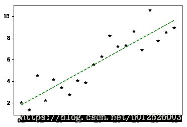
• 对于这种问题，最好需要将其归一化，否则SGD求解很容易发散。对于下面的例子，如果将X，即特征的范围取得非常大(比如下面range里面设置最大值为20之类的)，则求得的解很有可能就会发散。
• 除此之外，也有Lasso等加入正则化方法的线性回归

import matplotlib.pyplot as plt
import random as rnd
%matplotlib inline
import numpy as np
from pyspark.mllib.regression import LabeledPoint, LinearRegressionWithSGD, LassoWithSGD

x = np.linspace(0,4,20)
y = 2*x  + 2 + 4*np.random.random(x.shape)-2

data = sc.parallelize(np.column_stack( (x, y) ))

labeledData = data.map( lambda d : LabeledPoint(d[1] , d[0:1]) )
model = LinearRegressionWithSGD.train( labeledData, iterations=100, intercept=True )
y_pred = model.predict( np.array(x).reshape(1,-1) )
print( "weights : %s, intercept : %s" % (model.weights, model.intercept) )

plt.plot( x,y, 'k*', label="real" )
plt.plot( x,y_pred, 'g--', label="pred with intercept" )
plt.show()

weights : [1.960302173749138], intercept : 1.7728141318262047

Logistic Regression

• LR用于监督式分类问题，可以使用SGD等方法对LR进行训练，
• clearThreshold之后，LR会输出原始概率，也可以设置概率阈值，直接输出分类结果

from pyspark.mllib.classification import LogisticRegressionWithSGD

data = [LabeledPoint(0.0, [0.0, 1.0]), LabeledPoint(1.0, [1.0, 0.0])]
lrm = LogisticRegressionWithSGD.train( sc.parallelize(data), iterations=20 )
print( lrm.predict([1,0]) )
lrm.clearThreshold()
print( lrm.predict([1,0]) )
lrm.setThreshold(0.5)
print( lrm.predict([1,0]) )

1
0.7763929145707635
1

其他

• mllib同时也支持SVM、朴素贝叶斯、决策树、随机森林等机器学习方法

决策树的超参数

• data：由LabeledPoint组成的rdd
• numClasses：分类任务时，有该参数，表示类别数量
• impurity：节点的不纯度测量，对于分类可以使用gini系数或者信息熵，对回归只能是varainace
• maxDepth：数的最大深度，默认为5。
• maxBins：在构建各节点时，将数据分到多少个箱子中
• cateoricalFeaturesInfo：指定哪些特征是用于分类的，以及有多少个分类。

随机森林

除了上面的超参数之外，还有
* numTrees，即决策树的个数。
* featureSubsetStrategy：在每个节点上做决定时所考虑的特征的数量，可以是auto、all、sqrt、log2、onethird等，数目越大，计算的代价越大。
* seed：采用的随机数种子

聚类任务

• MLlib中包含kmeans以及kmeans||两种算法，后者可以为并行化环境提供更好的初始化策略。除了聚类的目标数量K之外，还包括以下几个超参数
• initializationMode：初始化聚类中心的方法，可以是kmeans||或者random。kmeans||的效果一般更好，但是更加耗时
• maxIterations：最大迭代次数，默认为100
• runs：算法并发运行的数目，mllib的kmeans支持从多个起点并发执行，然后选择最佳的结果。

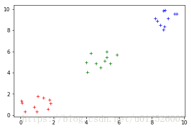
下面的代码中，首先训练一个kmeans模型，然后对其分类结果进行可视化

from pyspark.mllib.clustering import KMeans

data = 2*np.random.random((30, 2))
data[10:20,:] = data[10:20,:]+4
data[20:,:] = data[20:,:]+8

plt.plot( data[:,0], data[:,1], 'r+' )
plt.show()

rddData = sc.parallelize( data )
model = KMeans.train( rddData, 3, maxIterations=100, initializationMode="kmeans||",
                    seed=50, initializationSteps=5, epsilon=1e-4)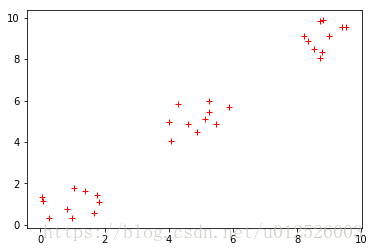

result = np.zeros((data.shape[0], ))
for ii in range( data.shape[0] ):
    result[ii] = model.predict( data[ii,:] )
colors = ["r+", "b+", "g+"]
for ii in range(3):
    plt.plot( data[result == ii, 0], data[result == ii, 1], colors[ii] )

plt.show()