深度学习(五) 生成对抗网络入门与实践
一.生成对抗网络基本概念
1.发展背景
自然界中人类的特性可以概括两大特殊能力,分别是认识和创造。那么在深度学习-神经网络中,我们之前所学习的全连接神经网络、卷积神经网络等,它们都有一个共同的特点就是只实现了认识的功能,或者说是分类。那么如何让网络能够具有创造力,能根据我们的需求去自主地创造呢?换句话说,我们想让一直当评委/裁判的神经网络,现在能够自己上台去表演。这就是生成对抗网络的由来。
生成式对抗网络(GAN, Generative Adversarial Networks )是一种深度学习模型,它在2014年由Ian Goodfellow首次提出,该模型通过框架中(至少)两个模块:生成模块(Generative Model)和判别模块(Discriminative Model)的互相博弈学习产生相当好的输出。随后几年里,GAN飞速发展,产生了广泛的应用。并衍生出了很多流行的模型变种,比如DCGAN、C-GAN、WGAN、pix2pix等等。
2.核心思想
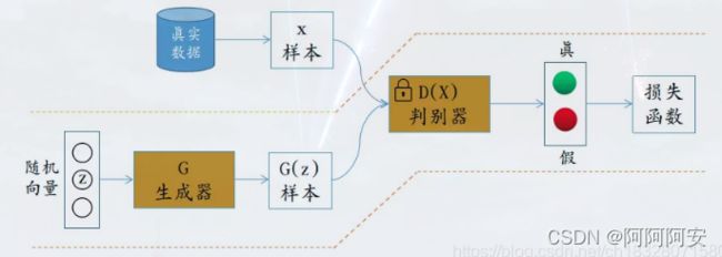
GAN主要由生成器模型G和判别器模型D两大模块组成,原始 GAN 理论中,并不要求 G 和 D 都是神经网络,只需要是能拟合相应生成和判别的函数即可。但实用中一般均使用不同结构的深度神经网络作为 G 和 D 。其中:
- 生成器模型G:生成器是用来创造样本的。其输入一些随机噪声,通过生成网络输出我们需要的样本数据(二维图像数据等)
- 判别器模型D:判别器是用来识别真假的。其输入生成器生成的样本和真实样本,通过判别网络输出对样本数据的真假分类判别(二分类)。
GAN受博弈论中的零和博弈启发,将生成问题视作判别器和生成器这两个网络的对抗和博弈:生成器从给定噪声中(一般是指均匀分布或者正态分布)产生合成数据,判别器分辨生成器的的输出和真实数据。前者试图产生更接近真实的数据,相应地,后者试图更完美地分辨真实数据与生成数据。由此,两个网络在对抗中进步,在进步后继续对抗,由生成式网络得的数据也就越来越完美,逼近真实数据,从而可以生成想要得到的数据(图片、序列、视频等),二者在不断的对抗中逐步到达一种纳什均衡状态。
通俗点来说:假如你(G)是一个初级绘画师,你想提高你的绘画能力达到世界大师的水平。但是只靠你自己是无法成功的,所以你叫来了你的朋友(D)帮助你。你们训练的方式就是:你不断创作绘画作品,然后将你的绘画作品和世界大师的作品一起交给你的朋友鉴赏,然后你的朋友来分辨哪一个是你画的,哪一个是大师的。
- 对于你来说:每次朋友鉴赏完成后,告诉你他的分辨结果。然后你根据结果不断改进自己不足的地方。目的就是不断提高自己的水平,让你朋友分辨不出来哪一个是你画的哪一个是大师的。
- 对于你朋友来说:每次你创作完成之后,要对你的进步负责。他都要尽可能正确的将大师作品和你画的作品区分开来,提高自己的鉴赏水平。
在你们两个不断地博弈对抗的过程中,你的绘画水平不断提高,甚至能达到以假乱真的效果。而你的朋友的鉴赏水平不断提高,甚至真画假画一眼便知。你们两个在对抗中一起成长,达到平衡。
二.训练过程
- 初始化生成器G和判别器D两个网络的初始参数。
- 固定生成器G的网络参数,从训练集抽取一个batch,生成器输入定义的随机噪声分布生成n个输出样本。
- 将真实训练样本数据与生成器输出样本数据拼接为判别器输入,并给以label真(1)和假(0),训练辨别器D,使其尽可能区分输入样本的真假。
- 这样循环训练更新k次判别器D之后,固定判别器参数。从训练集抽取一个batch,生成器输入定义的随机噪声分布生成n个输出样本。
- 将真实训练样本数据与生成器输出样本数据拼接为判别器输入,并给以label全真(1),训练辨别器D,使生成器输出的数据尽可能的真实,辨别器尽可能区分不了真假。
- 多轮这样的更新迭代后,理想状态下,最终辨别器D无法区分图片到底是来自真实的训练样本集合,还是来自生成器G生成的样本即可,此时辨别的概率为0.5,完成训练。或者达到相应的训练轮数阈值。

三.黑白图像着色问题实践
1.问题背景
黑白图像的彩色化问题一直以来都是研究的热点,该问题旨在输入黑白图像,输出着色彩色化后的彩色图像。对于此问题可以看作是一个色彩生成问题,我们可以借助GAN网络来进行解决。
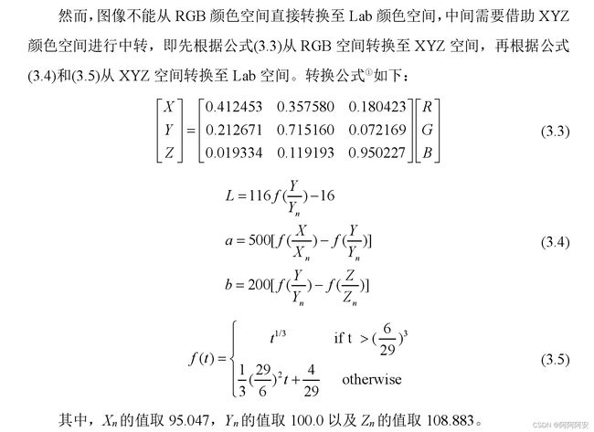
2.颜色空间
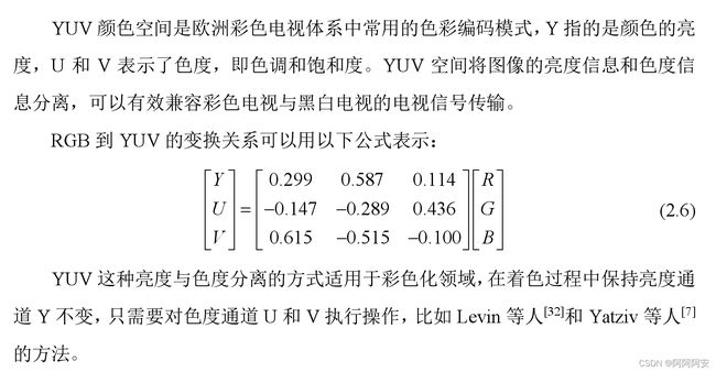
自然界中人们对于颜色的感受可以量化为色调、饱和度和亮度,其中色调表示颜色纯色的属性,比如红橙黄绿青蓝紫。饱和度表示色彩的鲜艳程度,纯色光越多饱和度越高,比如颜色的浓淡深浅。亮度描述颜色的明暗程度,可划分为黑灰白三个层次。颜色常用的量化定义分为三种类型,分别是RGB空间、YUV空间、Lab空间,三种颜色空间的说明如下:
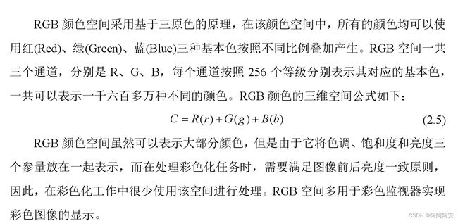
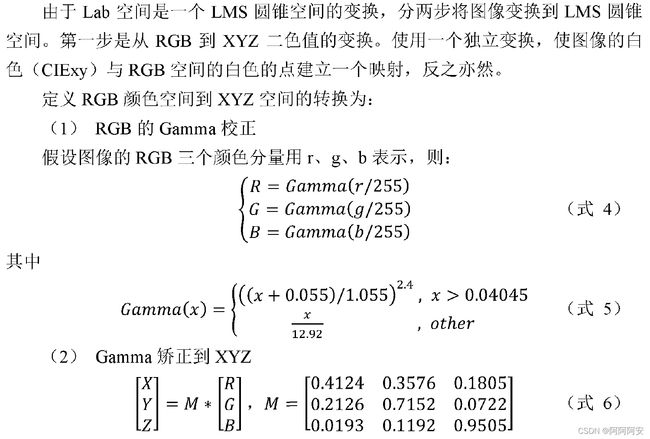
(1)RGB颜色空间 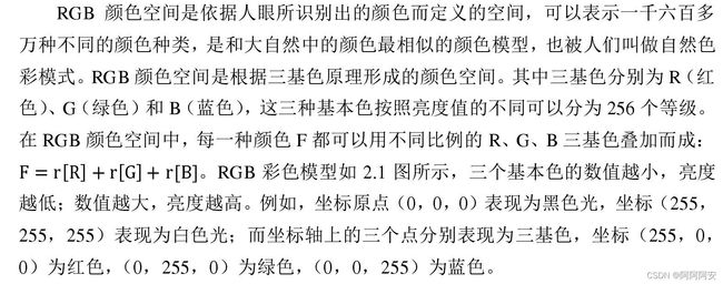
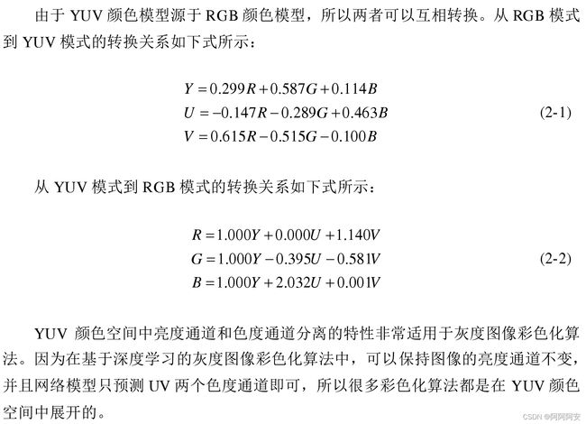
(2)YUV颜色空间
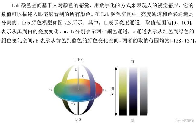
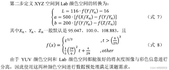
(3)Lab颜色空间
3.实验设计思路 (条件-生成对抗网络)
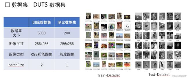
- 图片数据集导入(使用DUTS数据集)
- 图片数据处理:将导入的彩色rgb图像转换为Lab格式图像,按照训练集:测试集划分为5:1的比例,并将图像的L通道分量复制作为黑白图像噪声用于生成器神经网络输入训练
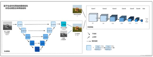
- 设计实现生成网络模型:使用改进的U-Net模型作为生成网络,输入为L通道分量的单通道黑白图像,输出为预测的a、b通道,叠加L通道分量后形成Lab格式的预测彩色图片
- 设计实现判别网络模型:输入真实图片和生成器预测图片拼接的数据集,输出预测标签(fake or true)
- 网络训练:每一轮先训练k次判别网络,固定生成网络;再训练一次生成网络,固定判别网络。如此反复多轮直到达到一定的阈值。
- 模型测试:使用训练好的生成模型,输入L通道的黑白图像,输出预测彩色图片
(1)数据集
(2) 模型结构
4.代码实现
(1)工具方法 util.py
import numpy as np
import torch
from skimage import color
from PIL import Image
import torchvision.transforms as transforms
from torchvision import utils

#从(h,w,c)格式的Lab中拿到 标准化的Tensor L通道、ab通道
def splitFromLab(image_lab):
    image_lab = image_lab.transpose((2, 0, 1)) #(c,h,w)
    image_l = image_lab[0]/100 #(h,w) L通道范围 0~100 -> 归一化到 0~1
    image_ab = image_lab[1:,:,:]/110 #(2,h,w) ab通道 -> 归一化到 -1~1
    image_l = torch.from_numpy(image_l).unsqueeze(0) #(1,h,w) Tensor
    image_ab = torch.from_numpy(image_ab) #(2,h,w) Tensor
    #返回标准化 L (1,h,w) + 真实图像lab(3,h,w)
    return image_l,torch.cat([image_l,image_ab],dim=0)

def TransfertToRGB(image):
    #image (1,3,h,w) -> (3,h,w)
    image = image.squeeze(0)
    image[0,:,:]*=100
    image[1:,:,:]*=110
    image_ndarray = np.array(image)
    #image (3,h,w) -> (h,w,3)
    image_lab = image_ndarray.transpose((1,2,0))
    #image rgb (h,w,3)
    image_rgb = color.lab2rgb(image_lab)
    #image rgb (1,3,h,w)
    image_rgb = torch.from_numpy(image_rgb.transpose((2, 0, 1))).unsqueeze(0)
    return image_rgb

def TransferBacktoWhite(path):
    transTensor = transforms.ToTensor()  # 将PIL Image自动转化并归一化为tensor(c,h,w)
    img_path = path
    image = Image.open(img_path).convert("RGB")  # 图片为 "RGB"格式 真彩图像 三通道 (h,w,c) 范围[0,255] -> 二值黑白图像.convert("1")
    image_tensor = transTensor(image)
    image_tensor[image_tensor>0.5] = 1
    image_tensor[image_tensor<=0.5] = 0
    save_path = r"D:\日常材料\图片照片\签名结果.png"
    # 注意,save_image将图像保存为RGB三通道,如果是二值图像则三个通道数值都相同,即伪灰度图像
    utils.save_image(image_tensor, save_path)

if __name__ == "__main__":
    path = r"D:\日常材料\图片照片\导师签名2.png"
    TransferBacktoWhite(path)
(2)数据集 data.py
import os
import numpy as np
from PIL import Image
from torch.utils.data import Dataset
from util import *
from skimage import color
os.environ["KMP_DUPLICATE_LIB_OK"]="TRUE"

#构造自定义数据集
class ModelDataset(Dataset):
    def __init__(self,image_dir):
        super(ModelDataset, self).__init__()
        self.image_dir = image_dir
        self.images = os.listdir(self.image_dir) #os.listdir()函数用于返回指定的文件夹包含的文件或文件夹的[名字]的列表。

    def __len__(self):
        return len(self.images)

    def __getitem__(self, index):
        #加载图片
        img_path = os.path.join(self.image_dir,self.images[index]) #os.path.join函数用于将字符串按照系统盘符拼接为路径
        image = Image.open(img_path).convert("RGB").resize((256,256)) #图片为 "RGB"格式 真彩图像 三通道 (h,w,c) 范围[0,255]
        # 图片转化为rgb Numpy (h,w,c)
        image_rgb = np.array(image)
        image_grey = np.array(image.convert("L"))/255
        # 将rgb空间 -> lab空间
        image_lab = color.rgb2lab(image_rgb)
        # 获取L、lab Tensor格式(c,h,w)归一化数据
        image_l,image_lab = splitFromLab(image_lab)
        return image_l,image_lab,torch.from_numpy(image_grey).unsqueeze(0)


'''
图片处理:
1.PIL
    (1)PIL读取数据:Image.open() 返回Image对象,尺寸为(width,height)
    (2)PIL显示图像:Image.show():调用本地的图片浏览器显示
    (3)PIL Image转换到Numpy ndarray:np.array(Image),尺寸为(height,width,channel)
    (4)matplotlib显示ndarry图像:plt.imshow(img)+plt.show() ,要求img尺寸为(H, W, C)
2.skimage
    (1)skimage读取数据:io.imread(img_path) ,返回ndarray格式,尺寸为(height,width,channel)
    (2)skimage显示图像:直接使用plt.show()显示ndarray
    (3)skimage颜色空间转换
        - rgb -> lab: color.rgb2lab(rgb, illuminant='D65', observer='2', *, channel_axis=- 1) 默认将(h,w,c)的rgb ndarray图像转化为(h,w,c)的lab图像
        - lab -> rgb: color.lab2rgb(lab, illuminant='D65', observer='2', *, channel_axis=- 1) 默认将(h,w,c)的lab ndarray图像转化为(h,w,c)的rgb图像
    (4)注意:
        - 对于rgb to lab来说:
            a.如果输入rgb为[0,255]的int类型,则在转换时,函数会先将输入/255转换到[0,1]之间的float64(这叫gamma矫正),再计算lab通道。
            b.如果输入rgb为[0,1]的/255之后的标准化float64数据,则函数不会进行处理,直接拿来计算lab
            c.函数最终返回float64 的 lab空间图像ndarray
            d.该函数就是严格按照rgb2lab公式来的:先->xyz->lab,要算gamma(r/255)矫正->lab等等,所以求出来的lab取值范围就是 L[0,100],a[-110,110],b[-110,110]
        - 对于lab to rgb来说:输入lab空间矩阵,返回[0,1]之间标准化的rgb颜色矩阵

3.Pytorch
    (1)神经网络中训练要求数据格式必须为 (channel,height,width)
    (2)格式转换1:torchvision.transforms.ToTensor 把一个取值范围是[0,255]的PIL.Image或者shape为(H,W,C)的numpy.ndarray,转换成形状为[C,H,W],取值范围是[0,1.0]的torch.FloatTensor(除以255,自动进行归一化)
    (3)格式转换2:交换维度np.transpose( xxx,  (2, 0, 1))  将xxx (H x W x C)的ndarray 转化为 (C x H x W)的ndarray
'''
(3)网络模型 net.py
import torch
import torch.nn as nn

#1.生成器-卷积模块
class ConvBlock(nn.Module):
    def __init__(self,in_channel,out_channel):
        super(ConvBlock, self).__init__()
        #构建 卷积块(进行两次卷积操作)
        self.layer = nn.Sequential(
            #第一次卷积操作
            nn.Conv2d(in_channel,out_channel,kernel_size=3,stride=1,padding=1),#卷积操作 (batch,in_ch,h,w) -> (batch,out_ch,h,w) 不改变大小
            nn.BatchNorm2d(out_channel),#批标准化 将数据标准化到正态分布
            nn.ReLU(inplace=True),#激活函数 inplace=True表示覆盖输入数据(避免了临时变量频繁释放,提高效率)
            #第二次卷积操作
            nn.Conv2d(out_channel, out_channel, kernel_size=3, stride=1, padding=1),
            # 卷积操作 (batch,in_ch,h,w) -> (batch,out_ch,h,w) 不改变大小
            nn.BatchNorm2d(out_channel),  # 批标准化 将数据标准化到正态分布
            nn.ReLU(inplace=True),  # 激活函数 inplace=True表示覆盖输入数据(避免了临时变量频繁释放,提高效率)
        )

    def forward(self,x):
        return self.layer(x)

#2.生成器-上采样模块:反卷积+拼接
class DeConvBlock(nn.Module):
    def __init__(self,in_channel,out_channel):
        super(DeConvBlock, self).__init__()
        #上采样:反卷积 (batch,in_ch,h,w) -> (batch,out_ch,2h,2w)
        self.up = nn.ConvTranspose2d(in_channel,out_channel,kernel_size=2,stride=2)

    def forward(self,input_1,input_2):
        output_2 = self.up(input_2) #先上采样
        merge = torch.cat([input_1,output_2],dim=1) #跳跃连接,合并输入
        return merge #返回合并后结果


#3.生成器网络
class Generator(nn.Module):
    def __init__(self,in_channel,out_channel):
        super(Generator, self).__init__()
        filter_maps = [64,128,256,512,1024]
        self.pool = nn.MaxPool2d(2)
        # 编码器
        self.encoderConv1 = ConvBlock(in_channel, filter_maps[0])
        self.encoderConv2 = ConvBlock(filter_maps[0], filter_maps[1])
        self.encoderConv3 = ConvBlock(filter_maps[1], filter_maps[2])
        self.encoderConv4 = ConvBlock(filter_maps[2], filter_maps[3])
        self.encoderConv5 = ConvBlock(filter_maps[3], filter_maps[4])
        # 解码器
        self.upSimple1 = DeConvBlock(filter_maps[4], filter_maps[3])
        self.decoderConv1 = ConvBlock(filter_maps[4], filter_maps[3])
        self.upSimple2 = DeConvBlock(filter_maps[3], filter_maps[2])
        self.decoderConv2 = ConvBlock(filter_maps[3], filter_maps[2])
        self.upSimple3 = DeConvBlock(filter_maps[2], filter_maps[1])
        self.decoderConv3 = ConvBlock(filter_maps[2], filter_maps[1])
        self.upSimple4 = DeConvBlock(filter_maps[1], filter_maps[0])
        self.decoderConv4 = ConvBlock(filter_maps[1], filter_maps[0])
        # 输出
        self.final = nn.Conv2d(filter_maps[0], out_channel, kernel_size=1)
        self.out = nn.Tanh()

    def forward(self, x):
        # 编码,下采样过程
        en_x1 = self.encoderConv1(x)  # 输出 (batch,64,256,256)
        down_x1 = self.pool(en_x1)  # 输出 (batch,64,128,128)
        en_x2 = self.encoderConv2(down_x1)  # 输出 (batch,128,128,128)
        down_x2 = self.pool(en_x2)  # 输出 (batch,128,64,64)
        en_x3 = self.encoderConv3(down_x2)  # 输出 (batch,256,64,64)
        down_x3 = self.pool(en_x3)  # 输出(batch,256,32,32)
        en_x4 = self.encoderConv4(down_x3)  # 输出(batch,512,32,32)
        down_x4 = self.pool(en_x4)  # 输出(batch,512,16,16)
        en_x5 = self.encoderConv5(down_x4)  # 输出(batch,1024,16,16)
        # 解码,上采样过程
        up_x1 = self.upSimple1(en_x4, en_x5)  # 输出 (batch,1024,32,32)
        de_x1 = self.decoderConv1(up_x1)  # 输出 (batch,512,32,32)
        up_x2 = self.upSimple2(en_x3, de_x1)  # 输出 (batch,512,64,64)
        de_x2 = self.decoderConv2(up_x2)  # 输出 (batch,256,64,64)
        up_x3 = self.upSimple3(en_x2, de_x2)  # 输出 (batch,256,128,128)
        de_x3 = self.decoderConv3(up_x3)  # 输出 (batch,128,128,128)
        up_x4 = self.upSimple4(en_x1, de_x3)  # 输出 (batch,128,256,256)
        de_x4 = self.decoderConv4(up_x4)  # 输出 (batch,64,256,256)
        # 输出
        return self.out(self.final(de_x4))  # 输出(batch,2,256,256) 图像ab通道 并标准化到(-1,1)

#4.判别器-卷积模块
class DiscriminatorBlock(nn.Module):
    def __init__(self,in_channel,out_channel):
        super(DiscriminatorBlock, self).__init__()
        #论文:使用stride=2来代替pool进行下采样,pool会损失信息!
        self.block = nn.Sequential(
            nn.Conv2d(in_channel, out_channel, kernel_size=4, stride=2, padding=1),
            nn.BatchNorm2d(out_channel),
            nn.LeakyReLU(0.2,inplace=True)
        )
    def forward(self,x):
        return self.block(x)

#5.判别器网络
class Discriminator(nn.Module):
    def __init__(self,in_channel):
        super(Discriminator, self).__init__()
        filter_maps = [32,64, 128, 256, 512]
        self.Conv1 = DiscriminatorBlock(in_channel,filter_maps[0])
        self.Conv2 = DiscriminatorBlock(filter_maps[0],filter_maps[1])
        self.Conv3 = DiscriminatorBlock(filter_maps[1],filter_maps[2])
        self.Conv4 = DiscriminatorBlock(filter_maps[2],filter_maps[3])
        self.Conv5 = DiscriminatorBlock(filter_maps[3],filter_maps[4])
        self.Conv6 = DiscriminatorBlock(filter_maps[4],filter_maps[4])
        self.out = nn.Conv2d(filter_maps[4],1,kernel_size=4,stride=1)
        self.cls = nn.Sigmoid()

    def forward(self,x):
        x = self.Conv1(x) #(b,32,128,128)
        x = self.Conv2(x) #(b,64,64,64)
        x = self.Conv3(x) #(b,128,32,32)
        x = self.Conv4(x) #(b,256,16,16)
        x = self.Conv5(x) #(b,512,8,8)
        x = self.Conv6(x) #(b,512,4,4)
        return self.cls(self.out(x)).view(-1) #(b,1,1,1) -> 一维(b)
(4)网络训练模块 train.py
import os
import torch
from torch.utils.data import DataLoader
from data import *
from net import *

device = torch.device('cuda' if torch.cuda.is_available() else 'cpu')#调整设备,优先使用gpu
img_dir = r"D:\日常材料\作业报告\机器学习\DUTS数据集\DUTS-TE\DUTS-TE-Image"
weightD_path = "params/Dnet.pth"
weightG_path = "params/Gnet.pth"
batch_size = 4
epoch = 10
d_every = 1
g_every = 2

if __name__ == "__main__":
    #1.加载自己训练数据集的数据加载器
    data_loader = DataLoader(ModelDataset(img_dir),batch_size=batch_size,shuffle=True)
    #2.将模型加载到设备上
    Dnet,Gnet = Discriminator(3).to(device),Generator(1,2).to(device)
    #2.1加载预训练权重(如果有的话)
    if os.path.exists(weightD_path):
        Dnet.load_state_dict(torch.load(weightD_path))
    if os.path.exists(weightG_path):
        Gnet.load_state_dict(torch.load(weightG_path))
    #3.设置优化器和损失
    optim_D = torch.optim.Adam(Dnet.parameters(),lr=0.0001,betas=(0.5,0.999))
    optim_G = torch.optim.Adam(Gnet.parameters(),lr=0.0001,betas=(0.5,0.999))
    criterion = torch.nn.BCELoss()
    #4.设置真假标签(真为1,假为0)
    true_label = torch.ones(batch_size).to(device)
    fake_label = torch.zeros(batch_size).to(device)
    #4.开始训练
    for i in range(epoch):
        lossSum_D = 0.0
        lossSum_G = 0.0

        for index,(img_l,img_real,_) in enumerate(data_loader):
            #img_l,img_real = img_l.to(device),img_real.to(device) #将数据放到设备上
            img_l,img_real = img_l.type(torch.cuda.FloatTensor).to(device),img_real.type(torch.cuda.FloatTensor).to(device)
            if index % d_every==0:
                #训练判别器,固定生成器
                #1.训练真实图片,尽可能将真图片判别为正确
                output_real = Dnet(img_real)
                loss_real = criterion(output_real,true_label)
                #累计梯度
                optim_D.zero_grad()
                loss_real.backward()
                #2.训练假图片,尽可能将假图片判别为假
                output_ab = Gnet(img_l).detach()#使用detach截断计算图,防止判别器更新生成器
                img_fake = torch.cat([img_l,output_ab],dim=1).to(device)
                output_fake = Dnet(img_fake)
                loss_fake = criterion(output_fake,fake_label)
                #累计梯度
                loss_fake.backward()
                #3.更新判别网络
                optim_D.step()
                lossSum_D = lossSum_D + loss_real.item() + loss_fake.item()
            if index % g_every==0:
                # 训练生成器,固定判别器
                # 1.生成假图片
                output_ab = Gnet(img_l)
                img_fake = torch.cat([img_l, output_ab], dim=1).to(device)
                output_fake = Dnet(img_fake)
                #2.让假图片尽可能以假乱真
                loss_fakeTrue = criterion(output_fake,true_label)
                #更新参数
                optim_G.zero_grad()
                loss_fakeTrue.backward()
                optim_G.step()
                lossSum_G = lossSum_G + loss_fakeTrue.item()

        torch.save(Dnet.state_dict(),weightD_path)#每一轮都保存训练参数weight
        torch.save(Gnet.state_dict(),weightG_path)
        print("[epoch %d]: Dloss is %.3f and Gloss is %.3f" % (i+1,lossSum_D,lossSum_G))
(5)网络测试模块 test.py
import os
import torch
from net import *
from data import *
from torch.utils.data import DataLoader
from torchvision import utils
from util import *
import matplotlib.pyplot as plt

image_dir = r"D:\日常材料\作业报告\机器学习\DUTS数据集\train_data"
save_dir = r"D:\日常材料\作业报告\机器学习\DUTS数据集\color_result"
weightG_path = "params/Gnet.pth"

Gnet = Generator(1,2)
if os.path.exists(weightG_path):
    Gnet.load_state_dict(torch.load(weightG_path))
    print("weights load successful")
else:
    print("weights is not exist")

Gnet.eval() #切换训练模式
test_loader = DataLoader(ModelDataset(image_dir),batch_size=1,shuffle=False) #(1,c,h,w) 网络必须四维输入

#不进行计算图构建
with torch.no_grad():
    for index,(test_img_l,test_img_real,test_img_grey) in enumerate(test_loader):
        test_img_l,test_img_real = test_img_l.type(torch.FloatTensor),test_img_real.type(torch.FloatTensor)
        out_ab = Gnet(test_img_l)
        out_image = torch.cat([test_img_l,out_ab],dim=1)
        image_grey = torch.cat([test_img_grey,test_img_grey,test_img_grey],dim=1)
        image_real = TransfertToRGB(test_img_real)
        image_color = TransfertToRGB(out_image)
        # 将真实图像和预测图象拼接(拼接到batch上,构造雪碧网格图),也可以降维输出单个图像
        img = torch.cat([image_grey,image_real,image_color],dim=0)
        #保存图像
        save_path = os.path.join(save_dir,str(index)+".png")
        #注意,save_image将图像保存为RGB三通道,如果是二值图像则三个通道数值都相同,即伪灰度图像
        utils.save_image(img,save_path)
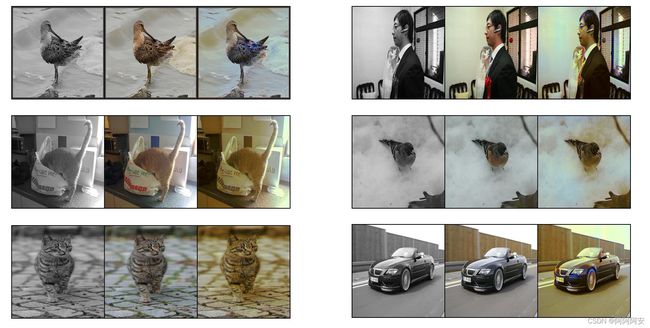
5.测试结果
从左到右依次是:黑白图像、原彩色图像、预测输出彩色图像。