线性回归模型

1常见机器学习概念

监督学习:通过标注数据进行学习的方法
无监督学习:当一组数据很难获取标签的时候采用无监督学习，一般采用的方法是聚类分析。
损失函数:一种衡量指标，用于衡量模型的预测偏离其标签的程度，在求解最优化问题的时候一般通过损失函数来对模型参数进行评估。
线性回归:一种通过属性的线性组合来进行预测的线性模型，其目的是找到一条直线或者一个平面或者更高维的超平面，使得预测值与真实值之间的误差最小化。
方差:表示一组数据的离散程度，

欠拟合:模型在训练集上指标不好并且在测试集上表现也不好，解决方法:增加特征、增加数据量，如1.例如，“组合”、“泛化”、“相关性”三类特征是特征添加的重要手段。2.添加多项式特征，这个在机器学习算法里面用的很普遍，例如将线性模型通过添加二次项或者三次项使模型泛化能力更强。3.减少正则化参数，正则化的目的是用来防止过拟合的，但是现在模型出现了欠拟合，则需要减少正则化参数。

过拟合:一个训练好的模型中训练集上指标很好而在测试集上表现不好，解决方法:减少特征、增加数据量。1.可能是数据不纯的原因，重新清洗数据2.采用正则化方法。正则化方法一般使用L1正则和L2正则，而正则一般是在目标函数之后加上对于的范数，L1正则(Lasso):各个参数绝对值之和，L2正则(岭回归):各个参数的平方和的开方值

泛化:指的是模型依据训练时采用的数据，针对以前未见过的新数据做出正确预测的能力。
交叉验证（cross-validation）:将原始数据进行分类分为训练集和测试集先对训练集中数据进行训练得到模型，在对测试集中数据用于验证，用于评价模型好坏。

2 线性回归算法

是什么?
一种通过属性的线性组合来进行预测的线性模型，其目的是找到一条直线或者一个平面或者更高维的超平面，使得预测值与真实值之间的误差最小化，一般分为一元线性回归与多元线性回归，公式为:Y=AX+B
一元线性回归模型公式是什么？如何推导?
在一个二维坐标系中一组数据变化可能呈 yi’ = a + bxi 这样的变化规律(如学历与工资、工作经验与工资)
如何求解一元线性回归模型?
使得|yi(真值)-yi’(预测值)|差距最小，则损失函数

线性回归损失函数:为了度量真值与预测值之间的差异需要计算J(x)的最小值,由于yi’ = a + bxi 则计算loss:

根据最小二乘法求出:分别对a,b求偏导




求偏导得出

代码实现
fit()函数封装了计算a，b的方法也就是上面两个公式，predict(array)函数传入x返回预测值y

 def __init__(self):
        '''初始化模型'''
        self.a_ = None
        self.b_ = None

    def fit(self,x_train,y_train):
        '''fit是用来求解线性回归模型的，
        将求出来的a,b计算公式写入'''
        assert x_train.ndim == 1, \
        "只处理一元线性回归情况，请输入一维数据"
        assert len(x_train) == len(y_train), \
        "x_train!==y_train"


        x_mean = np.mean(x_train)
        y_mean = np.mean(y_train)
        num = (x_train-x_mean).dot(y_train-y_mean)
    	d = (x_train-x_mean).dot(x_train-x_mean)
    	self.a_ = num / d
   		self.b_ = y_mean - self.a_ * x_mean

        return self

    def predect(self,x_predict):
        '''预测函数返回y向量结果'''
        assert x_predict.ndim == 1, \
            "只处理一元线性回归情况，请输入一维数据"
        assert self.a_ is not None and self.b_ is not None, \
            "必须知道ab的值"

        return np.array([self._predict(x) for x in x_predict])
    def _predict(self,x_single):
        '''对单个X_single进行预测返回预测值'''
        return self.a_ * x_single+self.b_
    def __repr__(self):
        return "DemoLinearRegression()"

效果如何:

import numpy as np
import matplotlib.pyplot as plt
from test_linar_reggestion.DemoLinearRegression import DemoLinearRegression
lin_reg = DemoLinearRegression()
x = np.array([1.,2.,3.,4.,5.,6.])
y = np.array([1.,3.,4.,2.,5.,6.])
plt.scatter(x,y)
plt.show()
a_b = lin_reg.fit(x,y)
print("a:",a_b.a_,"b:",a_b.b_)
reg1= a_b._predict(np.array([6]))
print(reg1)

结果为:a: 0.8285714285714286 b: 0.5999999999999996
[5.57142857]#预测值

什么是多元线性回归?
当数据有多个维度特征的时候如x1,x2,x3…,xn时求参数

公式为:

其中

目标函数:

接下来我们通过两种方法来求解线性回归模型的损失函数，
方法一:梯度下降

代码实现

import numpy as np
def error_function(theta, X, y):
    '''Error function J definition.'''
    diff = np.dot(X, theta) - y
    return (1. / 2 * len(X)) * np.dot(np.transpose(diff), diff)


def gradient_function(theta, X, y):
    '''Gradient of the function J definition.'''
    diff = np.dot(X, theta) - y
    return (1. / len(X)) * np.dot(np.transpose(X), diff)


def gradient_descent(X, y, alpha):
    '''Perform gradient descent.'''
    theta = np.array([1, 1]).reshape(2, 1)
    gradient = gradient_function(theta, X, y)
    while not np.all(np.absolute(gradient) <= 1e-5):
        theta = theta - alpha * gradient
        gradient = gradient_function(theta, X, y)
    return theta

进行测试

from test_linar_reggestion.gredient_descent import *

# Size of the points dataset.
m = 20

# Points x-coordinate and dummy value (x0, x1).
X0 = np.ones((m, 1))
X1 = np.arange(1, m+1).reshape(m, 1)
X = np.hstack((X0, X1))

# Points y-coordinate
y = np.array([
    3, 4, 5, 5, 2, 4, 7, 8, 11, 8, 12,
    11, 13, 13, 16, 17, 18, 17, 19, 21
]).reshape(m, 1)

# The Learning Rate alpha.
alpha = 0.01

optimal = gradient_descent(X, y, alpha)
print('optimal:', optimal)
print('error function:', error_function(optimal, X, y)[0,0])

结果:optimal: [[0.51583286]
[0.96992163]]
error function: 405.98496249324046
方法二:正规方程—最小二乘法
求解参数过程如下:

代码实现

import numpy as np
from test_linar_reggestion.score import r2_score
class LinearRression:
    def __init__(self):
        '''初始化模型'''
        self.coef_ = None
        self.interception_ = None
        self._theta = None

    def fie(self,x_train,y_train):
        '''训练模型'''
        assert x_train.shape[0] ==y_train.shape[0],\
            "维度相同"
        x_b = np.vstack([np.ones((len(x_train),1)),x_train])#添加x0行
        self._theta = np.linalg.inv(x_b.T.dot(x_b)).dot(x_b.T).dot(y_train)
        self.coef_ = self._theta[1:]
        self.interception_=self._theta[0]

        return self
    def predict(self,x_predict):
        x_b = np.vstack([np.ones((len(x_predict), 1)), x_predict])  # 添加x0行
        return x_b.dot(self._theta)
    def score(self,x_test,y_test):
        y_prdict = self.predict(x_test)
        return r2_score(y_test,y_prdict)

    def __repr__(self):
        return "LinearRression()"

线性回归的评估指标

yi与y’i分别指测试集中的真值与预测值。
平均绝对误差MAE(man Absolute Error)

均方误差MSE(mean Squared Error)

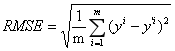
均方根误差RMSE(Root Mean Squared Error)

R^2

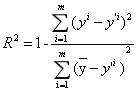
R^2是线性回归选择的评价标准
作用:衡量模型的拟合程度，
特点:1.小于等于1
2.越大越好，最优模型时r^2=1,也就是损失函数等于0
3.当训练模型等于基准模型的时候r^2=0
4.如果r^2<0说明训练模型不如基准模型
代码封装

import numpy as np
import pandas as pd
from math import sqrt

def mean_squared_error(y_test,y_predict):
    assert len(y_predict)== len(y_test), \
        "预测值与测试值数组大小必须相等"
    return np.average((y_predict-y_test)**2)
def root_mean_squared_error(y_test,y_predict):
    assert len(y_test) == len(y_predict), \
        "预测值与测试值数组大小必须相等"
    return sqrt(np.average((y_predict-y_test)**2))
def mean_absolute_error(y_test, y_predict):
    assert len(y_test) == len(y_predict), \
        "预测值与测试值数组大小必须相等"
    return np.average(np.absolute(y_test - y_predict))
def r2_score(y_test, y_predict):
    assert len(y_test) == len(y_predict), \
        "预测值与测试值数组大小必须相等"
    return 1-mean_squared_error(y_test, y_predict)/np.var(y_test)

sklearn参数详解

lin_reg.fit(x_train,y_train)#生成回归模型
lin_reg.coef_#存放回归系数
lin_reg.intercept_#存放截距
lin_reg.score(x,y)#评分函数，将返回一个小于1的得分，可能会小于0
lin_reg.predict(x_test)#预测值

fit()方法源码
判断数据是否规范

n_jobs_ = self.n_jobs
X, y = check_X_y(X, y, accept_sparse=['csr', 'csc', 'coo'],
                 y_numeric=True, multi_output=True)

if sample_weight is not None and np.atleast_1d(sample_weight).ndim > 1:
    raise ValueError("Sample weights must be 1D array or scalar")

X, y, X_offset, y_offset, X_scale = self._preprocess_data(
    X, y, fit_intercept=self.fit_intercept, normalize=self.normalize,
    copy=self.copy_X, sample_weight=sample_weight)

if sample_weight is not None:
    # Sample weight can be implemented via a simple rescaling.
    X, y = _rescale_data(X, y, sample_weight)

如果是简单矩阵行数<2直接使用sparse_lsqr(x,y)(#Sparse Equations and Least Squares)，否则使用进行迭代delayed(sparse_lsqr)(X, y[:, j].ravel())for j in range(y.shape[1]))。

   if sp.issparse(X):
                if y.ndim < 2:
                    out = sparse_lsqr(X, y)#通过sparse_lsqr函数来进行计算
                    self.coef_ = out[0]
                    self._residues = out[3]
                else:
                    # sparse_lstsq cannot handle y with shape (M, K)
                    outs = Parallel(n_jobs=n_jobs_)(
                        delayed(sparse_lsqr)(X, y[:, j].ravel())
                        for j in range(y.shape[1]))
                    self.coef_ = np.vstack(out[0] for out in outs)
                    self._residues = np.vstack(out[3] for out in outs)

lsqr()源码解析
第一步对数据进行处理

    def lsqr(A, b, damp=0.0, atol=1e-8, btol=1e-8, conlim=1e8,
             iter_lim=None, show=False, calc_var=False, x0=None):
    lin_reg.predict(x_test)#预测值
A = aslinearoperator(A)
    b = np.atleast_1d(b)
    if b.ndim > 1:
        b = b.squeeze()

    m, n = A.shape
    if iter_lim is None:
        iter_lim = 2 * n
    var = np.zeros(n)

    msg = ('The exact solution is  x = 0                              ',
         'Ax - b is small enough, given atol, btol                  ',
         'The least-squares solution is good enough, given atol     ',
         'The estimate of cond(Abar) has exceeded conlim            ',
         'Ax - b is small enough for this machine                   ',
         'The least-squares solution is good enough for this machine',
         'Cond(Abar) seems to be too large for this machine         ',
         'The iteration limit has been reached                      ')

    if show:
        print(' ')
        print('LSQR            Least-squares solution of  Ax = b')
        str1 = 'The matrix A has %8g rows  and %8g cols' % (m, n)
        str2 = 'damp = %20.14e   calc_var = %8g' % (damp, calc_var)
        str3 = 'atol = %8.2e                 conlim = %8.2e' % (atol, conlim)
        str4 = 'btol = %8.2e               iter_lim = %8g' % (btol, iter_lim)
        print(str1)
        print(str2)
        print(str3)
        print(str4)

源码解析
_decision_function()
将测试X传入return 到safe_sparse_dot中传入X、回归系数、截距

def _decision_function(self, X):
    check_is_fitted(self, "coef_")

    X = check_array(X, accept_sparse=['csr', 'csc', 'coo'])
    return safe_sparse_dot(X, self.coef_.T,
                           dense_output=True) + self.intercept_

看看safe_sparse_dot()源码，直接用通用矩阵乘法，尽量不要使用dot向量化点乘方法

def safe_sparse_dot(a, b, dense_output=False):
 

   """Dot product that handle the sparse matrix case correctly

    Uses BLAS GEMM as replacement for numpy.dot where possible
    to avoid unnecessary copies.

    Parameters
    ----------
    a : array or sparse matrix
    b : array or sparse matrix
    dense_output : boolean, default False
        When False, either ``a`` or ``b`` being sparse will yield sparse
        output. When True, output will always be an array.

    Returns
    -------
    dot_product : array or sparse matrix
        sparse if ``a`` or ``b`` is sparse and ``dense_output=False``.
    """
    if issparse(a) or issparse(b):
        ret = a * b
        if dense_output and hasattr(ret, "toarray"):
            ret = ret.toarray()
        return ret
    else:
        return np.dot(a, b)

score()函数可以看到sklearn中是用默认r^2来进行模型评估的，传入测试集当中的x_test,y_test返回 r^2_sorce

 def score(self, X, y, sample_weight=None):
        """Returns the coefficient of determination R^2 of the prediction.

        The coefficient R^2 is defined as (1 - u/v), where u is the residual
        sum of squares ((y_true - y_pred) ** 2).sum() and v is the total
        sum of squares ((y_true - y_true.mean()) ** 2).sum().
        The best possible score is 1.0 and it can be negative (because the
        model can be arbitrarily worse). A constant model that always
        predicts the expected value of y, disregarding the input features,
        would get a R^2 score of 0.0.

        Parameters
        ----------
        X : array-like, shape = (n_samples, n_features)
            Test samples.

        y : array-like, shape = (n_samples) or (n_samples, n_outputs)
            True values for X.

        sample_weight : array-like, shape = [n_samples], optional
            Sample weights.

        Returns
        -------
        score : float
            R^2 of self.predict(X) wrt. y.
        """

        from .metrics import r2_score
        return r2_score(y, self.predict(X), sample_weight=sample_weight,
                        multioutput='variance_weighted')

r2_score函数中对R^2公式算法进行封装并返回output_scores

def r2_score(y_true, y_pred, sample_weight=None,
             multioutput="uniform_average"):
  
    y_type, y_true, y_pred, multioutput = _check_reg_targets(
        y_true, y_pred, multioutput)

    if sample_weight is not None:
        sample_weight = column_or_1d(sample_weight)
        weight = sample_weight[:, np.newaxis]
    else:
        weight = 1.

    numerator = (weight * (y_true - y_pred) ** 2).sum(axis=0,
                                                      dtype=np.float64)
    denominator = (weight * (y_true - np.average(
        y_true, axis=0, weights=sample_weight)) ** 2).sum(axis=0,
                                                          dtype=np.float64)
    nonzero_denominator = denominator != 0
    nonzero_numerator = numerator != 0
    valid_score = nonzero_denominator & nonzero_numerator
    output_scores = np.ones([y_true.shape[1]])
    output_scores[valid_score] = 1 - (numerator[valid_score] /
                                      denominator[valid_score])
    # arbitrary set to zero to avoid -inf scores, having a constant
    # y_true is not interesting for scoring a regression anyway
    output_scores[nonzero_numerator & ~nonzero_denominator] = 0.
    if isinstance(multioutput, string_types):
        if multioutput == 'raw_values':
            # return scores individually
            return output_scores
        elif multioutput == 'uniform_average':
            # passing None as weights results is uniform mean
            avg_weights = None
        elif multioutput == 'variance_weighted':
            avg_weights = denominator
            # avoid fail on constant y or one-element arrays
            if not np.any(nonzero_denominator):
                if not np.any(nonzero_numerator):
                    return 1.0
                else:
                    return 0.0
    else:
        avg_weights = multioutput
return np.average(output_scores, weights=avg_weights)

实战项目boston房价预测及分析

导入相应的包并加载数据

import matplotlib.pyplot as plt
import numpy as np
from sklearn import datasets, linear_model, discriminant_analysis, cross_validation
from sklearn.linear_model import LinearRegression#导入线性回归包
boston = datasets.load_boston()
x = boston.data
y = boston.target
x= x[y<50]
y =y[y<50]

线性回归模型

from sklearn.linear_model import LinearRegression
lin_reg = LinearRegression()
lin_reg.fit(x,y)
print(lin_reg.coef_)

[-1.05574295e-01 3.52748549e-02 -4.35179251e-02 4.55405227e-01
-1.24268073e+01 3.75411229e+00 -2.36116881e-02 -1.21088069e+00
2.50740082e-01 -1.37702943e-02 -8.38888137e-01 7.93577159e-03
-3.50952134e-01]

对房价结果进行查看
print(boston.feature_names[np.argsort(lin_reg.coef_)])#按照负相关到正相关排序
print(boston.DESCR)

‘’’
[‘NOX’ ‘DIS’ ‘PTRATIO’ ‘LSTAT’ ‘CRIM’ ‘INDUS’ ‘AGE’ ‘TAX’ ‘B’ ‘ZN’ ‘RAD’
‘CHAS’ ‘RM’]
可以看到其中影响房价多个因素分别有负相关和正相关如下

		# 负相关		
		- NOX      nitric oxides concentration (parts per 10 million)#房子周边一氧化氮的浓度
		- DIS      weighted distances to five Boston employment centres#距离五个工作中心的距离
		- PTRATIO  pupil-teacher ratio by town#师生比例
	  	- LSTAT    % lower status of the population#人口地位
 		 - CRIM     per capita crime rate by town#犯罪率
        - INDUS    proportion of non-retail business acres per town#非零售业用地面积
        - AGE      proportion of owner-occupied units built prior to 1940#1940年以前建设的业主单位比例
        - TAX      full-value property-tax rate per $10,000#物业税
        
        #正相关
		-- B        1000(Bk - 0.63)^2 where Bk is the proportion of blacks by town#1000（bk-0.63）^2，其中bk是按城镇划分的黑人比例
        - ZN       proportion of residential land zoned for lots over 25,000 sq.ft.#住宅用地比例
         - RAD      index of accessibility to radial highways放射性公路的达标指标
        - CHAS     Charles River dummy variable (= 1 if tract bounds river; 0 otherwise)#charles river这条河附近的房子
		- RM       average number of rooms per dwelling#房间数量
'''