@线性回归模型
原文地址:http://www.seyvoue.com/posts/91fff0b1/
声明:版权所有,转载请联系作者并注明出
overview: linear regression with one variable or multiple variables, gradient descent, normal equation, feature scaling, contour plot.
Example
| Input x | Output y |
|---|---|
| 0 | 2 |
| 1 | 4 |
| 2 | 6 |
| 3 | 8 |
从表中的数据,可以用 hθ(x)=2+2x ,拟合表中的数据。
于是当给定一个新的输入,如 x=4 ,可以预测出输出 y=2+2∗4=10
一元线性回归
建模
Hypothesis:
Cost Function:
Gradient Descent:
其中,公式 (1-3) 即,
repeatuntilconvergence:{
}
另外, α 为 learning rate.
应用
该实例来源于 coursera machine learning programming exercise1.
- DataSet
数据集的部分内容如下,完整数据集在这里。
| Population of a city (x) | Profit of a food truck in that city (y) |
|---|---|
| 6.1101 | 17.592 |
| 5.5277 | 9.1302 |
| 8.5186 | 13.662 |
| … | … |
- 目的:
如果你需要在别的城市开一家分店,经过调查,你发现利润与城市的人口有关,现需要根据已掌握的数据,去预测在 A 市开分店的收益会如何?(即告诉你 A 市的人口,利用拟合出的模型,去预测可能的利润)
完整代码
完整代码可在这里下载。
下面只列出其中的主程序:
%% Linear regression with one variable
% x refers to the population size in 10,000s
% y refers to the profit in $10,000s
%

%% Initialization
clear ; close all; clc

%% ==================== Part 1: Basic Function ====================
% Complete warmUpExercise.m
fprintf('Running warmUpExercise ... \n');
fprintf('5x5 Identity Matrix: \n');
warmUpExercise()

fprintf('Program paused. Press enter to continue.\n');
pause;


%% ======================= Part 2: Plotting =======================
fprintf('Plotting Data ...\n')
data = load('ex1data1.txt');
X = data(:, 1); y = data(:, 2);
m = length(y); % number of training examples

% Plot Data
% Note: You have to complete the code in plotData.m
plotData(X, y);

fprintf('Program paused. Press enter to continue.\n');
pause;

%% =================== Part 3: Cost and Gradient descent ===================

X = [ones(m, 1), data(:,1)]; % Add a column of ones to x
theta = zeros(2, 1); % initialize fitting parameters

% Some gradient descent settings
iterations = 1500;
alpha = 0.01;

fprintf('\nTesting the cost function ...\n')
% compute and display initial cost
J = computeCost(X, y, theta);
fprintf('With theta = [0 ; 0]\nCost computed = %f\n', J);
fprintf('Expected cost value (approx) 32.07\n');

% further testing of the cost function
J = computeCost(X, y, [-1 ; 2]);
fprintf('\nWith theta = [-1 ; 2]\nCost computed = %f\n', J);
fprintf('Expected cost value (approx) 54.24\n');

fprintf('Program paused. Press enter to continue.\n');
pause;

fprintf('\nRunning Gradient Descent ...\n')
% run gradient descent
theta = gradientDescent(X, y, theta, alpha, iterations);

% print theta to screen
fprintf('Theta found by gradient descent:\n');
fprintf('%f\n', theta);
fprintf('Expected theta values (approx)\n');
fprintf(' -3.6303\n  1.1664\n\n');

% Plot the linear fit
hold on; % keep previous plot visible
plot(X(:,2), X*theta, '-')
legend('Training data', 'Linear regression')
hold off % don't overlay any more plots on this figure

% Predict values for population sizes of 35,000 and 70,000
predict1 = [1, 3.5] *theta;
fprintf('For population = 35,000, we predict a profit of %f\n',...
    predict1*10000);
predict2 = [1, 7] * theta;
fprintf('For population = 70,000, we predict a profit of %f\n',...
    predict2*10000);

fprintf('Program paused. Press enter to continue.\n');
pause;

%% ============= Part 4: Visualizing J(theta_0, theta_1) =============
fprintf('Visualizing J(theta_0, theta_1) ...\n')

% Grid over which we will calculate J
theta0_vals = linspace(-10, 10, 100);
theta1_vals = linspace(-1, 4, 100);

% initialize J_vals to a matrix of 0's
J_vals = zeros(length(theta0_vals), length(theta1_vals));

% Fill out J_vals
for i = 1:length(theta0_vals)
    for j = 1:length(theta1_vals)
      t = [theta0_vals(i); theta1_vals(j)];
      J_vals(i,j) = computeCost(X, y, t);
    end
end


% Because of the way meshgrids work in the surf command, we need to
% transpose J_vals before calling surf, or else the axes will be flipped
J_vals = J_vals';
% Surface plot
figure;
surf(theta0_vals, theta1_vals, J_vals)
xlabel('\theta_0'); ylabel('\theta_1');

% Contour plot
figure;
% Plot J_vals as 15 contours spaced logarithmically between 0.01 and 100
contour(theta0_vals, theta1_vals, J_vals, logspace(-2, 3, 20))
xlabel('\theta_0'); ylabel('\theta_1');
hold on;
plot(theta(1), theta(2), 'rx', 'MarkerSize', 10, 'LineWidth', 2);
代码分步讲解
- step1: 绘制散点图,观察训练集的数据分布。
data = load('ex1data1.txt');
X = data(:, 1); y = data(:, 2);
m = length(y); % number of training examples

figure; % open a new figure window
plot(x,y,'rx','MarkerSize',10);
xlabel('Population of City in 10,000s');
ylabel('Profit in $10,000s');
- step2: Computing cost function J(θ)
X = [ones(m, 1), data(:,1)]; % Add a column of ones to x
theta = zeros(2, 1); % initialize fitting parameters

% Some gradient descent settings
iterations = 1500;
alpha = 0.01;

fprintf('\nTesting the cost function ...\n')
% compute and display initial cost
J = computeCost(X, y, theta);
fprintf('With theta = [0 ; 0]\nCost computed = %f\n', J);
fprintf('Expected cost value (approx) 32.07\n');

% further testing of the cost function
J = computeCost(X, y, [-1 ; 2]);
fprintf('\nWith theta = [-1 ; 2]\nCost computed = %f\n', J);
fprintf('Expected cost value (approx) 54.24\n');
上面代码中的 computeCost(X, y, theta) 函数的代码如下:
function J = computeCost(X, y, theta)
%COMPUTECOST Compute cost for linear regression
%   J = COMPUTECOST(X, y, theta) computes the cost of using theta as the
%   parameter for linear regression to fit the data points in X and y

m = length(y); % number of training examples

J = 0;
h = X * theta;
for i=1:m,
    J = J + (h(i)-y(i))^2;
end;
J = J/(2*m);

end- step3: 用 gradient descent 找到 J(θ) 的最优解 (θ0,θ1)
本例中即找出合适的 (θ0,θ1) ,使得 J(θ) 最小(或者说在允许的差值范围内)
fprintf('\nRunning Gradient Descent ...\n')
% run gradient descent
theta = gradientDescent(X, y, theta, alpha, iterations);

% print theta to screen
fprintf('Theta found by gradient descent:\n');
fprintf('%f\n', theta);
上面代码中 gradientDescent(X, y, theta, alpha, iterations) 函数的代码如下:
function [theta, J_history] = gradientDescent(X, y, theta, alpha, num_iters)
%GRADIENTDESCENT Performs gradient descent to learn theta
%   theta = GRADIENTDESCENT(X, y, theta, alpha, num_iters) updates theta by
%   taking num_iters gradient steps with learning rate alpha

% Initialize some useful values
m = length(y); % number of training examples
J_history = zeros(num_iters, 1);

for iter = 1:num_iters,
    theta = theta - X' * alpha / m * (X *theta - y);
    % Save the cost J in every iteration
    J_history(iter) = computeCost(X, y, theta);
end

end- step4: 绘制拟合出的线性回归模型 hθ(x)
% Plot the linear fit
hold on; % keep previous plot visible
plot(X(:,2), X*theta, '-')
legend('Training data', 'Linear regression')
hold off % don't overlay any more plots on this figure
- step5: 预测
预测分店开在人口为 35,000 and 70,000 城市的利润
predict1 = [1, 3.5] *theta;
fprintf('For population = 35,000, we predict a profit of %f\n',...
    predict1*10000);
predict2 = [1, 7] * theta;
fprintf('For population = 70,000, we predict a profit of %f\n',...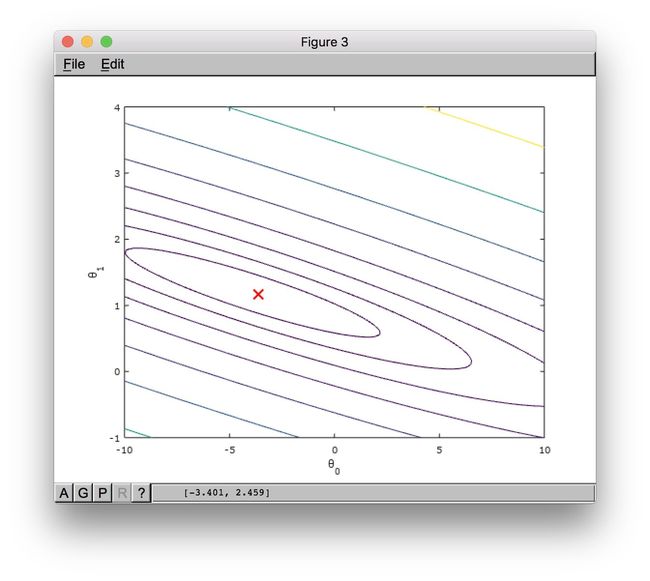
predict2*10000);- (optional)step6: 绘制 J(θ) 。观察其在不同 (θ0,θ1) 下的值
fprintf('Visualizing J(theta_0, theta_1) ...\n')

% Grid over which we will calculate J
theta0_vals = linspace(-10, 10, 100);
theta1_vals = linspace(-1, 4, 100);

% initialize J_vals to a matrix of 0's
J_vals = zeros(length(theta0_vals), length(theta1_vals));

% Fill out J_vals
for i = 1:length(theta0_vals)
    for j = 1:length(theta1_vals)
      t = [theta0_vals(i); theta1_vals(j)];
      J_vals(i,j) = computeCost(X, y, t);
    end
end

% Because of the way meshgrids work in the surf command, we need to
% transpose J_vals before calling surf, or else the axes will be flipped
J_vals = J_vals';
% Surface plot
figure;
surf(theta0_vals, theta1_vals, J_vals)
xlabel('\theta_0'); ylabel('\theta_1');

% Contour plot
figure;
% Plot J_vals as 15 contours spaced logarithmically between 0.01 and 100
contour(theta0_vals, theta1_vals, J_vals, logspace(-2, 3, 20))
xlabel('\theta_0'); ylabel('\theta_1');
hold on;
plot(theta(1), theta(2), 'rx', 'MarkerSize', 10, 'LineWidth', 2);
多元线性回归
建模
非向量形式写法
Hypothesis:
h_{\theta}(x)=\theta_0+\theta_1x+\theta_2x+\cdots+\theta_nx_n
\tag{2-1}\label{2-1}Cost Function:
J(\theta)=\frac{1}{2m}\sum_{i=1}^{m}(h_\theta(x^{(i)})-y^{(i)})^2
\tag{2-2}\label{2-2}Gradient Descent:
\theta_j:=\theta_j-\alpha\frac{\partial}{\partial\theta_j}J(\theta)
\quad for \, j=1..n
\tag{2-3}\label{2-3}
公式 (2-3) 即:
repeatuntilconvergence:{
}
⇔
repeatuntilconvergence:{
}
向量形式写法
- 公式 (2-1) 的向量形式:
\tag{2-1'}\label{2-1-1}
推导过程如下:
先看看当训练集只有一条记录时,向量形式如何表达,
当训练集有 m 条记录时,即可得到公式 (2-1') ,
令
- 公式 (2-2) 的向量形式:
\tag{2-2'}\label{2-2-1}
- 公式 (2-3) 的向量形式:
\tag{2-3'}\label{2-3-1}
推导过程如下:
⇒
另外, α 为 learning rate.
应用
该实例来源于 coursera machine learning programming exercise1.
已知:
- DataSet
数据集的部分内容如下,完整数据集在这里
| Size of the house (x1) | Number of bedrooms (x2) | Price of the house |
|---|---|---|
| 2104 | 3 | 399900 |
| 1600 | 3 | 329900 |
| 2400 | 3 | 369900 |
| 1416 | 2 | 232000 |
| … | … | … |
- 目的:
若房价与房子的面积,房间的数量有关,作为房东的你,想要预测手上已有房源的市场价。
完整代码
完整代码可在这里下载。
下面只列出其中的主程序:
%% Linear regression with multiple variables

%% Initialization

%% ================ Part 1: Feature Normalization ================

%% Clear and Close Figures
clear ; close all; clc

fprintf('Loading data ...\n');

%% Load Data
data = load('ex1data2.txt');
X = data(:, 1:2);
y = data(:, 3);
m = length(y);

% Print out some data points
fprintf('First 10 examples from the dataset: \n');
fprintf(' x = [%.0f %.0f], y = %.0f \n', [X(1:10,:) y(1:10,:)]');

fprintf('Program paused. Press enter to continue.\n');
pause;

% Scale features and set them to zero mean
fprintf('Normalizing Features ...\n');

[X mu sigma] = featureNormalize(X);

% Add intercept term to X
X = [ones(m, 1) X];


%% ================ Part 2: Gradient Descent ================

% ====================== YOUR CODE HERE ======================
% Instructions: We have provided you with the following starter
%               code that runs gradient descent with a particular
%               learning rate (alpha).
%
%               Your task is to first make sure that your functions -
%               computeCost and gradientDescent already work with
%               this starter code and support multiple variables.
%
%               After that, try running gradient descent with
%               different values of alpha and see which one gives
%               you the best result.
%
%               Finally, you should complete the code at the end
%               to predict the price of a 1650 sq-ft, 3 br house.
%
% Hint: By using the 'hold on' command, you can plot multiple
%       graphs on the same figure.
%
% Hint: At prediction, make sure you do the same feature normalization.
%

fprintf('Running gradient descent ...\n');

% Choose some alpha value
alpha = 0.01;
num_iters = 400;

% Init Theta and Run Gradient Descent
theta = zeros(3, 1);
[theta, J_history] = gradientDescentMulti(X, y, theta, alpha, num_iters);

% Plot the convergence graph
figure;
plot(1:numel(J_history), J_history, '-b', 'LineWidth', 2);
xlabel('Number of iterations');
ylabel('Cost J');

% Display gradient descent's result
fprintf('Theta computed from gradient descent: \n');
fprintf(' %f \n', theta);
fprintf('\n');

% Estimate the price of a 1650 sq-ft, 3 br house
% ====================== YOUR CODE HERE ======================
% Recall that the first column of X is all-ones. Thus, it does
% not need to be normalized.
price = featureNormalize([1 1650 3]) * theta; % You should change this


% ============================================================

fprintf(['Predicted price of a 1650 sq-ft, 3 br house ' ...
         '(using gradient descent):\n $%f\n'], price);

fprintf('Program paused. Press enter to continue.\n');
pause;

%% ================ Part 3: Normal Equations ================

fprintf('Solving with normal equations...\n');

% ====================== YOUR CODE HERE ======================
% Instructions: The following code computes the closed form
%               solution for linear regression using the normal
%               equations. You should complete the code in
%               normalEqn.m
%
%               After doing so, you should complete this code
%               to predict the price of a 1650 sq-ft, 3 br house.
%

%% Load Data
data = csvread('ex1data2.txt');
X = data(:, 1:2);
y = data(:, 3);
m = length(y);

% Add intercept term to X
X = [ones(m, 1) X];

% Calculate the parameters from the normal equation
theta = normalEqn(X, y);

% Display normal equation's result
fprintf('Theta computed from the normal equations: \n');
fprintf(' %f \n', theta);
fprintf('\n');


% Estimate the price of a 1650 sq-ft, 3 br house
% ====================== YOUR CODE HERE ======================
price = [1 1650 3] * theta; % You should change this


% ============================================================

fprintf(['Predicted price of a 1650 sq-ft, 3 br house ' ...
         '(using normal equations):\n $%f\n'], price);
代码分步讲解
- step1: 特征的归一化处理 feature normalization
data = load('ex1data2.txt');
X = data(:, 1:2);
y = data(:, 3);
m = length(y);

% Scale features and set them to zero mean
fprintf('Normalizing Features ...\n');

[X mu sigma] = featureNormalize(X);

% Add intercept term to X
X = [ones(m, 1) X];
代码中的 featureNormalize(X) 函数如下:
function [X_norm, mu, sigma] = featureNormalize(X)
%FEATURENORMALIZE Normalizes the features in X
%   FEATURENORMALIZE(X) returns a normalized version of X where
%   the mean value of each feature is 0 and the standard deviation
%   is 1. This is often a good preprocessing step to do when
%   working with learning algorithms.

% You need to set these values correctly
X_norm = X;
mu = zeros(1, size(X, 2));
sigma = zeros(1, size(X, 2));

% Instructions: First, for each feature dimension, compute the mean
%               of the feature and subtract it from the dataset,
%               storing the mean value in mu. Next, compute the
%               standard deviation of each feature and divide
%               each feature by it's standard deviation, storing
%               the standard deviation in sigma.
%
%               Note that X is a matrix where each column is a
%               feature and each row is an example. You need
%               to perform the normalization separately for
%               each feature.
%
% Hint: You might find the 'mean' and 'std' functions useful.
%

mu = mean(X);
sigma = std(X);
for i = 1:size(X,1),
    X_norm(i,:) = (X_norm(i,:)-mu) ./ sigma;
end;

end- step2: 用 gradient descent 找到 J(Θ) 的最优解 Θ
fprintf('Running gradient descent ...\n');

% Choose some alpha value
alpha = 0.01;
num_iters = 400;

% Init Theta and Run Gradient Descent
theta = zeros(3, 1);
[theta, J_history] = gradientDescentMulti(X, y, theta, alpha, num_iters);

% Display gradient descent's result
fprintf('Theta computed from gradient descent: \n');
fprintf(' %f \n', theta);
fprintf('\n');代码中的gradientDescentMulti(X, y, theta, alpha, num_iters)函数代码如下:
function [theta, J_history] = gradientDescentMulti(X, y, theta, alpha, num_iters)
%GRADIENTDESCENTMULTI Performs gradient descent to learn theta
%   theta = GRADIENTDESCENTMULTI(x, y, theta, alpha, num_iters) updates theta by
%   taking num_iters gradient steps with learning rate alpha

% Initialize some useful values
m = length(y); % number of training examples
J_history = zeros(num_iters, 1);

for iter = 1:num_iters,
    theta = theta - X' * alpha / m * (X *theta - y);
    % Save the cost J in every iteration
    J_history(iter) = computeCostMulti(X, y, theta);
end

end代码中的computeCostMulti(X, y, theta)函数代码如下:
function J = computeCostMulti(X, y, theta)
%COMPUTECOSTMULTI Compute cost for linear regression with multiple variables
%   J = COMPUTECOSTMULTI(X, y, theta) computes the cost of using theta as the
%   parameter for linear regression to fit the data points in X and y

% Initialize some useful values
m = length(y); % number of training examples

% You need to return the following variables correctly
J = 0;

h = X * theta;
for i=1:m,
    J = J + (h(i)-y(i))^2;
end;
J = J/(2*m);

end- step3: 绘制 J(Θ) 关于迭代次数的曲线图,以帮助选择合适的 learning rate α
% Plot the convergence graph
figure;
plot(1:numel(J_history), J_history, '-b', 'LineWidth', 2);
xlabel('Number of iterations');
ylabel('Cost J');
- step4: 预测
预测 size=1650(feet2),bedrooms=3 的房价。
% Estimate the price of a 1650 sq-ft, 3 br house
price = featureNormalize([1 1650 3]) * theta; %其中的 theta 在之前几步已经算出- (Optional)也可以使用 Normal Equation 代替 gradient descent 去寻找最优解
fprintf('Solving with normal equations...\n');

%% Load Data
data = csvread('ex1data2.txt');
X = data(:, 1:2);
y = data(:, 3);
m = length(y);

% Add intercept term to X
X = [ones(m, 1) X];

% Calculate the parameters from the normal equation
theta = normalEqn(X, y);

% Display normal equation's result
fprintf('Theta computed from the normal equations: \n');
fprintf(' %f \n', theta);
fprintf('\n');代码中的normalEqn(X, y)函数代码如下:
function [theta] = normalEqn(X, y)
%NORMALEQN Computes the closed-form solution to linear regression
%   NORMALEQN(X,y) computes the closed-form solution to linear
%   regression using the normal equations.

theta = zeros(size(X, 2), 1);
theta = pinv(X' * X) * X' * y;

end
Note:
使用 normal equation,相比于 gradient descent 来说代码量更小。
| Gradient Descent | Normal Equation |
|---|---|
| need to choose learning rate ‘ α ’ | No need to choose learning rate ‘ α ’ |
| needs many iterations | No need to iterate |
| 时间复杂度 O(kn2) | 时间复杂度 O(n3) |
| works well when n is large(n = nums of features) | slow if n is very large |