时间序列R语言操作——非平稳时间序列变平稳
文章目录
- 前言
- 一、方差不平稳
- 二、具有趋势性
-
- 1、确定性趋势的删除——趋势拟合法
- 2、随机趋势的删除——差分法
- 3、未知趋势的删除——平滑法
-
- 1. 移动平均法
- 2. 指数平滑法
- 4、季节性
-
- 1.Method1: 减掉趋势成分后取平均
- 2.Method2:使用哑元变量做回归分析
前言
时间序列为什么要平稳后建模?
- 时间序列是平稳的,则没有任何预测价值,因为均值不变,所以实际上人们只会对非平稳时间序列感兴趣
- 之所以研究平稳时间序列,因为总希望可以通过差分等方式把非平稳序列变成平稳的,而平稳时间序列可以通过数学公式予以解释
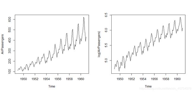
一、方差不平稳
最简单的是做对数变换,使得前后方差没有那么变化。
#Log transform: variance stationary
data(AirPassengers)
AirPassengers
par(mfrow=c(1,2))
plot(AirPassengers)
plot(log(AirPassengers))
二、具有趋势性
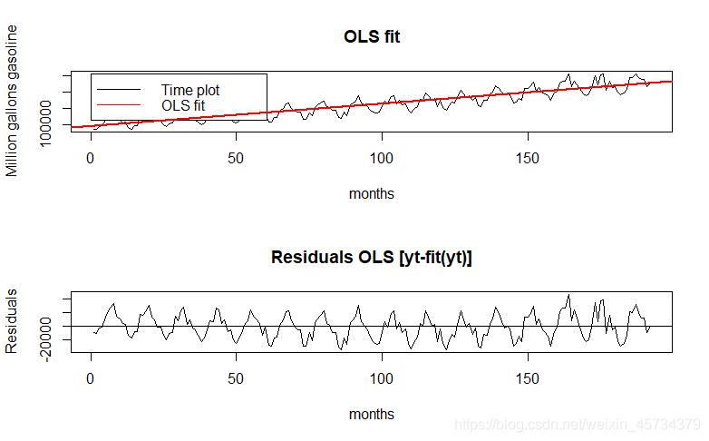
1、确定性趋势的删除——趋势拟合法
最简单的处理方法就是考虑均值函数可以由一个时间的确定性函数来描述,比如可以用回归模型来描述。对于一个有线性趋势的序列,可以做一个线性模型。
- Linear trend
##read the gasline data
##Abraham and Ledolter (1983) on the
##monthly gasoline demand in Ontario over the period 1960 - 1975.
gas = scan("gas.dat")
## note that read.table() would give an error here since the data is not in rectangular format.
gas.ts = ts(gas, frequency = 12, start = 1960)
gas.ts
plot(gas.ts, main = "Gasoline demand in Ontario", ylab = "Million gallons")
#fit trend:OLS with constant and trend
time = 1:length(gas.ts)
fit = lm(gas.ts~time)
summary(fit)#R-squared:  0.8225
par(mfrow=c(2,1))
plot(time, gas.ts, type='l', xlab='months', ylab='Million gallons gasoline',
main="OLS fit")
legend(.1, 256000, c("Time plot", "OLS fit"), col = c(1,2), text.col = "black",
merge = TRUE, lty=c(1,1))
abline(fit,col=2,lwd=2)
plot(time, fit$resid, type='l', xlab="months", ylab="Residuals",main="Residuals OLS [yt-fit(yt)]")
abline(a=0, b=0)#残差在0附近点波动
#savePlot("plot of Residuals_gas",type="pdf")
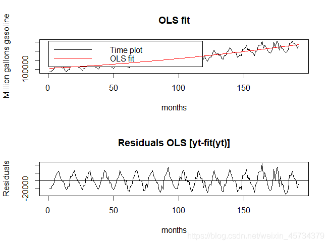
- Quadratic trend
fit2 = lm(gas.ts~time+I(time^2))
summary(fit2)#R-squared:  0.8327
names(fit2)
par(mfrow=c(2,1))
plot(time, gas.ts, type='l', xlab='months', ylab='Million gallons gasoline',
     main="OLS fit")
legend(.1, 256000, c("Time plot", "OLS fit"), col = c(1,2), text.col = "black",
       merge = TRUE, lty=c(1,1))
lines(time,fitted(fit2),col=2)
plot(time, fit2$resid, type='l', xlab="months", ylab="Residuals",main="Residuals OLS [yt-fit(yt)]")
abline(a=0, b=0)
- Polynomial trend
2、随机趋势的删除——差分法
随机趋势的删除——差分法。
- 一阶差分可以使线性趋势的序列实现趋势平稳
Zt = as.ts(rnorm(1000, sd = 20))
RW1 = as.ts(cumsum(Zt))
par(mfrow = c(2,2))
plot(RW1, main = "Random walk")
acf(RW1, main = "Correlogram random walk")
Yt=as.ts(diff(RW1))
plot(Yt,main='Diff(RW1)')
acf(Yt)

- 序列蕴含着曲线趋势,通常低阶(二阶或三阶)差分可提取出曲线趋势的影响 ,这里效果不好的话,可以先取对数,再做差分
- 对于蕴含着固定周期的序列进行步长为周期长度的差分运算,通常可以较好地提取周期信息
- 差分的阶数要适度,避免过差分
3、未知趋势的删除——平滑法
平滑法——顾名思义,使序列变平滑。 期望结果,是显示出趋势变化的规律。
1. 移动平均法
假定在短的时间间隔内,序列的取值是比较稳定的,序列的大小差异主要是由随机波动造成的。用一段时间间隔内的平均值作为某一期的估计值。
- 简单移动平均
##Moving average Model
Vt5 = filter(Zt, rep(1/5, 5), sides = 2)
Vt21 = filter(Zt, rep(1/21, 21), sides = 2)
par(mfrow = c(2,2))
plot(Vt5, main = "Moving 5-point average of above white noise series")
acf(Vt5, main = "Correlogram 5-point moving average", lag.max = 40, na.action = na.pass)
plot(Vt21, main = "Moving 21-point average of above white noise series")
acf(Vt21, main = "Correlogram 21-point moving average", lag.max = 40, na.action = na.pass)
par(mfrow = c(1,1))

- 权重移动平均
2. 指数平滑法
4、季节性
Seasonality means an effect that happens at the same time and with the same magnitude and direction every year. 从而使得经过季节调整的序列能够较好的反应社会经济指标运行基本态势。
1.Method1: 减掉趋势成分后取平均
## Investigating seasonality
library(fields)
z = matrix(fit$resid, ncol=12, byrow=TRUE)
colnames(z) = c("Jan","Feb","Mar","Apr","May","Jun","Jul","Aug","Sep","Oct","Nov","Dec")
bplot(z, xlab="Month", ylab="Detrended demand of gasoline", main="Annual seasonality of the detrended demand of gasoline")
mean=matrix(0, nrow=ncol(z), ncol=1) #mean for each month
for(i in 1:ncol(z)){
  mean[i,1]=mean(z[,i])
}
Seas = as.matrix(rep(mean,16)) # matrix with seasonal term
des.gas = fit$resid - Seas   # detrended and now deseasonized series
par(mfrow=c(2,1))
plot(fit$resid, type='l', xlab="months", ylab="Residuals", main="Residuals OLS [yt-fit(yt)]")
abline(a=0, b=0)
plot(des.gas, type='l', xlab="months", ylab="Deseasonized residuals", main="Deseasonized ResidualsOLS")
abline(a=0, b=0)

2.Method2:使用哑元变量做回归分析
##seasonal modeling and estimating seasonal trends
##such as for the average monthly temperature data
library(TSA)  #install package TSA
win.graph(width=4.875, height=2.5,pointsize=8)
data(tempdub);
plot(tempdub,ylab='Temperature',type='o')
month.=season(tempdub) # period added to improve table display
model2=lm(tempdub~month.) # -1 removes the intercept term
summary(model2)
Call:
lm(formula = tempdub ~ month.)

Residuals:
    Min      1Q  Median      3Q     Max
-8.2750 -2.2479  0.1125  1.8896  9.8250

Coefficients:
                Estimate Std. Error t value Pr(>|t|)
(Intercept)       16.608      0.987  16.828  < 2e-16 ***
month.February     4.042      1.396   2.896  0.00443 **
month.March       15.867      1.396  11.368  < 2e-16 ***
month.April       29.917      1.396  21.434  < 2e-16 ***
month.May         41.483      1.396  29.721  < 2e-16 ***
month.June        50.892      1.396  36.461  < 2e-16 ***
month.July        55.108      1.396  39.482  < 2e-16 ***
month.August      52.725      1.396  37.775  < 2e-16 ***
month.September   44.417      1.396  31.822  < 2e-16 ***
month.October     34.367      1.396  24.622  < 2e-16 ***
month.November    20.042      1.396  14.359  < 2e-16 ***
month.December     7.033      1.396   5.039 1.51e-06 ***
---
Signif. codes:  0 ‘***’ 0.001 ‘**’ 0.01 ‘*’ 0.05 ‘.’ 0.1 ‘ ’ 1

Residual standard error: 3.419 on 132 degrees of freedom
Multiple R-squared:  0.9712,	Adjusted R-squared:  0.9688
F-statistic: 405.1 on 11 and 132 DF,  p-value: < 2.2e-16