Pytorch之EfficientNetv1图像分类

---

• 个人主页:风间琉璃
• 版权: 本文由【风间琉璃】原创、在CSDN首发、需要转载请联系博主
• 如果文章对你有帮助、欢迎关注、点赞、收藏(一键三连)和订阅专栏哦

---

前言

EfficientNet是2019年google提出的网络模型，在论文提出了一种多维度混合的模型放缩方法，它通过利用Neural Architecture Search (NAS)技术，同时考虑输入分辨率、网络深度和网络宽度，构建更优秀的网络结构。EfficientNet的作者提供了8个网络模型，其中EfficientNet-B0是最基础的模型，EfficientNet-B1至B7是在B0的基础上通过NAS搜索技术进行了综合调整，调整内容包括输入分辨率、网络深度和网络宽度。

---

一、EfficientNet V1

1.EfficientNet简介

作者希望找到一个可以同时兼顾速度与精度的模型放缩方法，为此，作者重新审视了前人提出的模型放缩的几个维度：网络深度、网络宽度、图像分辨率，前人的文章多是放大其中的一个维度以达到更高的准确率，比如 ResNet-18 到 ResNet-152 是通过增加网络深度的方法来提高准确率。

作者跳出了前人对放缩模型的理解，从一个高度去审视这些放缩维度。作者认为 这三个维度之间是互相影响的并探索出了三者之间最好的组合，在此基础上提出了最新的网络 EfficientNet，该网络的表现如下：

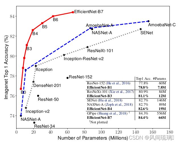
图中红色曲线为EfficientNet B7，横轴为模型大小，纵轴为准确率。对于ImageNet历史上的各种网络而言，可以说EfficientNet在效果上实现了碾压。

2.compound scaling methed（模型复合缩放方法）

一般在扩展网络的时候，一般通过调成输入图像的大小、网络深度和网络宽度（卷积通道数）。但是在EfficientNet之前，研究工作只是针对这三个维度中的某一个维度进行调整，很少有研究对这三个维度进行综合调整的。

EfficientNet的设想就是能否设计一个标准化的卷积网络扩展方法，既可以实现较高的准确率，又可以充分的节省算力资源。因而问题可以描述成，如何平衡分辨率、深度和宽度这三个维度，来实现网络在效率和准确率上的优化。

EfficientNet提出的解决方案是 模型复合缩放方法 (compound scaling methed)。

图(a)是一个基线网络，图(b)-(d)是传统的缩放方法，只增加网络宽度、网络深度和图像分辨率的其中一个维度。图(e)是作者提出的复合缩放方法，以一个固定的比例统一缩放所有三个维度。

在之前的论文中，有的会通过增加网络的width即增加卷积核的个数（增加特征矩阵的channels）来提升网络的性能如图(b)所示，有的会通过增加网络的深度，即使用更多的层结构来提升网络的性能如图©所示，有的会通过增加输入网络的分辨率来提升网络的性能如图(d)所示。

而在本篇论文中会同时增加网络的width、网络的深度以及输入网络的分辨率来提升网络，如图(e)所示。

根据以往的经验，增加网络的深度depth能够得到更加丰富、复杂的特征并且能够很好的应用到其它任务中。 但网络的深度过深会面临梯度消失，训练困难的问题。 增加网络的width能够获得 更高细粒度的特征并且也更容易训练，但对于 width很大而深度较浅的网络往往很难学习到更深层次的特征。 增加输入网络的图像分辨率能够潜在得获得 更高细粒度的特征模板，但对于非常高的输入分辨率， 准确率的增益也会减小。并且大分辨率图像会增加计算量。

上图展示了在基准EfficientNetB-0上分别增加width、depth以及resolution后得到的统计结果。通过上图可以看出大概在Accuracy达到80%时就趋于饱和了。

采用不同的depth，resolution组合，然后不断改变网络的width就得到如下图所示的4条曲线，通过分析可以发现在相同的FLOPs下，同时增加depth和resolution的效果最好。

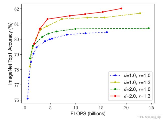
从实验结果来看，最高精度相比之前已经有所提升，突破了80%。而且组合不同，效果不同。作者又得到了一个观点：得到了更高的精度以及效率的关键是平衡网络的宽度，网络深度，网络分辨率三个维度的缩放倍率。

将整个卷积网络称为 N，它的第 i 个卷积层可以看作是下面的函数映射：Y_i = F_i(X_i) ，Y_i为输出张量，X_i为输入张量，设其维度为i，W_i，C_i>，为了简便省略了batch维度，则整个卷积网络N，由k个卷积层组成，可以表示为：
$$N(d，w，r)=F_k⨀\cdot \cdot \cdot ⨀F_2⨀F_1(X_1)=\underset{j=\mathrm{1...}k}{⨀}{F}_j(X_1)$$

通常降多个结构相同的卷积层称为一个stage，以stage为单位可以降卷积网络N表示为：
$$N(d，w，r)=\underset{i=\mathrm{1...}s}{⨀}{F}_i^{L_i}(X_{<H_i，W_i，C_i>})$$
其中：
$\star$ ${⨀}_{i=\mathrm{1...}s}$表示连乘运算，下标从1到s表示stage的序号。
$\star$ $F_i^{L_i}$表示第i个stage，它由卷积层$F_i$重复$F_i$次构成，$F_i$表示一个运算操作。
$\star$ $⟨H_i，W_i，C_i⟩$ 表示stage输入tensor的维度，即X的高度，宽度以及Channel。

为了减小搜索空间，作者固定了网络的基本结构，而只变动上面提到的三个放缩维度，网络深度(Li)，网络宽度(Ci)，输入分辨率大小(Hi, Wi)。尽管只搜索这三个维度，搜索空间依然很大，因此作者又加了一个限制，网络的放大只能在初识网络(EfficientNet-B0)的基础上乘上常数倍率，那么只需要优化w、d、r 分别是网络宽度，网络高度，分辨率的倍率，以此抽象出最终的数学模型：
$$\underset{d,w,r}{\max }Accuracy(N(d,w,r))$$ $$s.tN(d,w,r)={\odot }_{i=\mathrm{1...}s}{F}_i^{d\cdot L_i}(X_{⟨r\cdot H_i，r\cdot W_i，w\cdot C_i⟩})$$ $$Memory(N)\le targe{t}_{m}emory$$ $$FLOPs(N)\le targe{t}_{f}lops(2)$$
其中：
$\star$ d用来缩放深度$L_i$
$\star$ r用来缩放分辨率，即影响$H_i和W_i$
$\star$ w用来缩放特征矩阵的channel，即$C_i$
$\star$ target_memory为memory限制
$\star$ traget_flops为FLOPs限制

由此，作者提出了一种混合维度放大法(compound scaling method)，该方法 使用一个混合系数$\Phi$来决定缩放width，depth，resolution三个维度的放大倍率 ，具体的计算公式如下，其中s.t.代表限制条件：
$$depth:d={\alpha }^{\Phi }$$ $$width:w={\beta }^{\Phi }$$ $$resolution:r={\gamma }^{\Phi }(3)$$ $$s.t.\alpha \cdot {\beta }^2\cdot {\gamma }^2\approx 2$$ $$\alpha \ge 1,\beta \ge 1,\gamma \ge 1$$
其中， $\alpha ,\beta ,\gamma$均为常数(不是无限大的因为三者对应了计算量)，可通过网格搜索获得。混合系数$\Phi$可以人工调节。考虑到如果网络深度depth翻番那么对应计算量FLOPs会翻番，而网络宽度wideh或者图像分辨率resolution翻番对应计算量FLOPs会翻 4 番，即卷积操作的计算量(FLOPS) 与$d,w^2,r^2$成正比，因此上图中的约束条件中有两个平方项。在该约束条件下，指定混合系数$\Phi$之后，网络的计算量FLOPs大约是之前的$2^{\Phi }$倍。

卷积层FLOPs = $featur{e}_w\times featur{e}_h\times featur{e}_c\times kerne{l}_w\times kerne{l}_h\times kerne{l}_{nember}$

接下来作者在基准网络EfficientNetB-0上使用NAS来搜索$\alpha ,\beta ,\gamma$,

①首先固定复合系数$\Phi =1$，并基于上面给出的公式(2)和(3)进行搜索，作者发现对于EfficientNetB-0最佳参数为$\alpha =1.2,\beta =1.1,\gamma =1.15$
②接着固定$\alpha =1.2,\beta =1.1,\gamma =1.15$，通过复合调整公式对基线网络进行扩展，在EfficientNetB-0的基础上使用不同的$\Phi$分得到EfficientNetB-1至EfficientNetB-7参数

3.MBConv结构

MBConv结构是EfficientNet网络中堆叠的基本单元。(类似于Mobilenetv3中的block)，如下图所示MBConv结构。

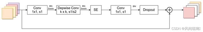
MBConv结构主要由一个1x1的普通卷积（升维作用，包含BN和Swish），一个k x k的Depthwise Conv卷积（包含BN和Swish），k的具体值可看EfficientNet-B0的网络框架主要有3x3和5x5两种情况，一个SE模块，一个1x1的普通卷积（降维作用，包含BN），一个Droupout层构成。

其中，第一个升维的1x1卷积层，它的卷积核个数是输入特征矩阵channel的n倍，n ∈ {1，6}。当n = 1时，不要第一个升维的1x1卷积层，即Stage2中的MBConv结构都没有第一个升维的1x1卷积层（这和MobileNetV3网络类似）。

关于shortcut连接，仅当输入MBConv结构的特征矩阵与输出的特征矩阵shape相同时才存在。

SE模块如下所示，由一个全局平均池化，两个全连接层组成。第一个全连接层的节点个数是输入该MBConv特征矩阵channels的$\frac{1}{4}$，且使用Swish激活函数。第二个全连接层的节点个数等于Depthwise Conv层输出的特征矩阵channels，且使用Sigmoid激活函数。

Dropout层 的dropout_rate对应的是drop_connect_rate，和全连接层对应的dropout要区分开，在源码实现中只有使用shortcut且drop_rate大于0 的时候才有Dropout层。

4.网络结构

EfficientNet作者给了8个网络，以EfficientNet-B0为例进行介绍，因为EfficientNet-B1~B7是在EfficientNet-B0的基础上，利用NAS搜索技术，对输入分辨率Resolution、网络深度Layers、网络宽度Channels三者进行综合调整。

EfficientNet-B0的网络结构，如下表所示

EfficientNet-B0的网络框架，总体看，分成了9个Stage：

①Stage1 是一个卷积核大小为3x3，步距为2的普通卷积层（包含BN和激活函数Swish）
②Stage2～Stage8 是在重复堆叠 MBConv 结构
③Stage9 是一个1x1的卷积层(包含BN和激活函数Swish) + 一个平均池化层 + 一个全连接层组成

表格中每个参数解析：

①表格中每个MBConv后会跟一个数字，1或6是倍率因子n (channel的倍数)，即MBConv中第一个1x1的卷积层会将输入特征矩阵的channels扩充为n倍。
②表格中k3x3或k5x5 表示MBConv中Depthwise Conv所采用的卷积核大小。
③Resolution表示该Stage的输入channel尺寸。
④Channels表示通过该Stage后输出特征矩阵的Channels。
⑤Layers表示该Stage重复MBConv结构多少次

通过上面的内容，可以搭建出EfficientNetB0网络的，其他版本的详细参数可见下表：

表格中每个参数解析：
$\star$ input_size 代表网络训练时输入图像大小

$\star$ width_coefficient 代表channel维度上的倍率因子，比如在 EfficientNetB0中Stage1的3x3卷积层所使用的卷积核个数是32，那么在B6中就是32 × 1.8 = 57.6，接着取整到离它最近的8的整数倍即56，其它Stage同理。

$\star$ depth_coefficient 代表depth维度上的倍率因子（仅针对Stage2到Stage8），比如在EfficientNetB0中Stage7中的MBConv6重复4次(Layers=4)，则在B6中Layers=4 × 2.6 = 10.4 ，向上取整即11。

$\star$ drop_connect_rate 是在 MBConv结构中dropout层使用的drop_rate，MBConv结构的drop_rate是从0递增到drop_connect_rate的。在MBConv中的Dropout层表示随机丢掉整个block的主分支，只剩shortcut分支，相当于直接跳过了这个block，可以理解为减少了网络的深度。

$\star$ dropout_rate是最后一个全连接层前的dropout层（在stage9的Pooling与FC之间）的dropout_rate。

二、EfficientNet V1网络实现

1.构建EfficientNetV1网络

import math
import copy
from functools import partial
from collections import OrderedDict
from typing import Optional, Callable

import torch
import torch.nn as nn
from torch import Tensor
from torch.nn import functional as F


def _make_divisible(ch, divisor=8, min_ch=None):
    """
    This function is taken from the original tf repo.
    It ensures that all layers have a channel number that is divisible by 8
    It can be seen here:
    https://github.com/tensorflow/models/blob/master/research/slim/nets/mobilenet/mobilenet.py
    """
    if min_ch is None:
        min_ch = divisor
    new_ch = max(min_ch, int(ch + divisor / 2) // divisor * divisor)
    # Make sure that round down does not go down by more than 10%.
    if new_ch < 0.9 * ch:
        new_ch += divisor
    return new_ch


def drop_path(x, drop_prob: float = 0., training: bool = False):
    """
    Drop paths (Stochastic Depth) per sample (when applied in main path of residual blocks).
    "Deep Networks with Stochastic Depth", https://arxiv.org/pdf/1603.09382.pdf

    This function is taken from the rwightman.
    It can be seen here:
    https://github.com/rwightman/pytorch-image-models/blob/master/timm/models/layers/drop.py#L140
    """
    if drop_prob == 0. or not training:
        return x
    keep_prob = 1 - drop_prob
    shape = (x.shape[0],) + (1,) * (x.ndim - 1)  # work with diff dim tensors, not just 2D ConvNets
    random_tensor = keep_prob + torch.rand(shape, dtype=x.dtype, device=x.device)
    random_tensor.floor_()  # binarize
    output = x.div(keep_prob) * random_tensor
    return output


class DropPath(nn.Module):
    """
    Drop paths (Stochastic Depth) per sample  (when applied in main path of residual blocks).
    "Deep Networks with Stochastic Depth", https://arxiv.org/pdf/1603.09382.pdf
    """
    def __init__(self, drop_prob=None):
        super(DropPath, self).__init__()
        self.drop_prob = drop_prob

    def forward(self, x):
        return drop_path(x, self.drop_prob, self.training)


# 处理流程：conv-->BN-->Activation(默认SiLU(Swish))
class ConvBNActivation(nn.Sequential):
    def __init__(self,
                 in_planes: int,
                 out_planes: int,
                 kernel_size: int = 3,
                 stride: int = 1,
                 groups: int = 1,
                 norm_layer: Optional[Callable[..., nn.Module]] = None,
                 activation_layer: Optional[Callable[..., nn.Module]] = None):
        padding = (kernel_size - 1) // 2
        # 默认使用
        if norm_layer is None:
            norm_layer = nn.BatchNorm2d
        if activation_layer is None:
            activation_layer = nn.SiLU  # SiLU 就是 alias Swish  (torch>=1.7)

        super(ConvBNActivation, self).__init__(nn.Conv2d(in_channels=in_planes,
                                                         out_channels=out_planes,
                                                         kernel_size=kernel_size,
                                                         stride=stride,
                                                         padding=padding,
                                                         groups=groups,
                                                         bias=False),
                                               norm_layer(out_planes),
                                               activation_layer())


# SE模块
class SqueezeExcitation(nn.Module):
    def __init__(self,
                 input_c: int,   # block input channel
                 expand_c: int,  # block expand channel
                 squeeze_factor: int = 4):
        super(SqueezeExcitation, self).__init__()
        # 第一个全连接层的个数
        squeeze_c = input_c // squeeze_factor
        # 卷积层代替全连接层
        self.fc1 = nn.Conv2d(expand_c, squeeze_c, 1)
        self.ac1 = nn.SiLU()  # alias Swish
        self.fc2 = nn.Conv2d(squeeze_c, expand_c, 1)
        self.ac2 = nn.Sigmoid()

    def forward(self, x: Tensor) -> Tensor:
        scale = F.adaptive_avg_pool2d(x, output_size=(1, 1))
        scale = self.fc1(scale)
        scale = self.ac1(scale)
        scale = self.fc2(scale)
        scale = self.ac2(scale)
        return scale * x


# MBConv模块配置参数
class InvertedResidualConfig:
    # kernel_size, in_channel, out_channel, exp_ratio, strides, use_SE, drop_connect_rate
    def __init__(self,
                 kernel: int,          # 3 or 5
                 input_c: int,
                 out_c: int,
                 expanded_ratio: int,  # 1 or 6
                 stride: int,          # 1 or 2
                 use_se: bool,         # True
                 drop_rate: float,
                 index: str,           # 1a, 2a, 2b, ... 层名称
                 width_coefficient: float):  # 网络宽度倍率因子
        # incput_c = input_c * width_coefficient，这里做了优化，为最近8的整数倍
        self.input_c = self.adjust_channels(input_c, width_coefficient)
        self.kernel = kernel
        self.expanded_c = self.input_c * expanded_ratio
        self.out_c = self.adjust_channels(out_c, width_coefficient)
        self.use_se = use_se
        self.stride = stride
        self.drop_rate = drop_rate
        self.index = index

    @staticmethod
    def adjust_channels(channels: int, width_coefficient: float):
        return _make_divisible(channels * width_coefficient, 8)


# MBConv模块
class InvertedResidual(nn.Module):
    def __init__(self,
                 cnf: InvertedResidualConfig,
                 norm_layer: Callable[..., nn.Module]):
        super(InvertedResidual, self).__init__()

        if cnf.stride not in [1, 2]:
            raise ValueError("illegal stride value.")

        # 关于shortcut连接，stride=1且当输入MBConv结构的特征矩阵与输出的特征矩阵，shape相同时才存在
        self.use_res_connect = (cnf.stride == 1 and cnf.input_c == cnf.out_c)

        # 有序的字典
        layers = OrderedDict()
        activation_layer = nn.SiLU  # alias Swish

        # expand
        if cnf.expanded_c != cnf.input_c:
            layers.update({"expand_conv": ConvBNActivation(cnf.input_c,
                                                           cnf.expanded_c,
                                                           kernel_size=1,
                                                           norm_layer=norm_layer,
                                                           activation_layer=activation_layer)})

        # depthwise
        layers.update({"dwconv": ConvBNActivation(cnf.expanded_c,
                                                  cnf.expanded_c,
                                                  kernel_size=cnf.kernel,
                                                  stride=cnf.stride,
                                                  groups=cnf.expanded_c,
                                                  norm_layer=norm_layer,
                                                  activation_layer=activation_layer)})

        if cnf.use_se:
            layers.update({"se": SqueezeExcitation(cnf.input_c,
                                                   cnf.expanded_c)})

        # project：最后一层1x1卷积
        layers.update({"project_conv": ConvBNActivation(cnf.expanded_c,
                                                        cnf.out_c,
                                                        kernel_size=1,
                                                        norm_layer=norm_layer,
                                                        activation_layer=nn.Identity)})
        # 主分支网络结构
        self.block = nn.Sequential(layers)
        self.out_channels = cnf.out_c
        self.is_strided = cnf.stride > 1

        # 只有在使用shortcut连接时才使用dropout层
        if self.use_res_connect and cnf.drop_rate > 0:
            self.dropout = DropPath(cnf.drop_rate)
        else:
            self.dropout = nn.Identity()

    def forward(self, x: Tensor) -> Tensor:
        result = self.block(x)
        result = self.dropout(result)
        if self.use_res_connect:  # shortcut分支
            result += x

        return result


class EfficientNet(nn.Module):
    def __init__(self,
                 width_coefficient: float,         # channel维度上的倍率因子
                 depth_coefficient: float,         # depth维度上的倍率因子
                 num_classes: int = 1000,
                 dropout_rate: float = 0.2,        # 最后一个全连接层前的dropout层（在stage9的Pooling与FC之间）的dropout_rate
                 drop_connect_rate: float = 0.2,   # MBConv结构中dropout层使用的drop_rate
                 block: Optional[Callable[..., nn.Module]] = None,
                 norm_layer: Optional[Callable[..., nn.Module]] = None
                 ):
        super(EfficientNet, self).__init__()

        # kernel_size, in_channel, out_channel, exp_ratio, strides, use_SE, drop_connect_rate, repeats
        # 配置表：EfficientNet-B0
        default_cnf = [[3, 32, 16, 1, 1, True, drop_connect_rate, 1],  # stage2
                       [3, 16, 24, 6, 2, True, drop_connect_rate, 2],
                       [5, 24, 40, 6, 2, True, drop_connect_rate, 2],
                       [3, 40, 80, 6, 2, True, drop_connect_rate, 3],
                       [5, 80, 112, 6, 1, True, drop_connect_rate, 3],
                       [5, 112, 192, 6, 2, True, drop_connect_rate, 4],
                       [3, 192, 320, 6, 1, True, drop_connect_rate, 1]]  # stage8

        def round_repeats(repeats):
            """Round number of repeats based on depth multiplier. 向上取整"""
            return int(math.ceil(depth_coefficient * repeats))

        if block is None:
            block = InvertedResidual

        if norm_layer is None:
            # 创建一个新函数，将参数eps固定为1e-3，momentum=0.1
            norm_layer = partial(nn.BatchNorm2d, eps=1e-3, momentum=0.1)

        adjust_channels = partial(InvertedResidualConfig.adjust_channels,
                                  width_coefficient=width_coefficient)

        # build inverted_residual_setting
        bneck_conf = partial(InvertedResidualConfig,
                             width_coefficient=width_coefficient)

        b = 0  # 目前总的搭建次数
        # stage重复次数
        num_blocks = float(sum(round_repeats(i[-1]) for i in default_cnf))
        inverted_residual_setting = []
        # 遍历同时获取索引和值
        for stage, args in enumerate(default_cnf):
            cnf = copy.copy(args)
            # 遍历stage中MBConv模块
            for i in range(round_repeats(cnf.pop(-1))):
                if i > 0:
                    # strides equal 1 except first cnf
                    cnf[-3] = 1  # strides
                    cnf[1] = cnf[2]  # input_channel equal output_channel

                cnf[-1] = args[-2] * b / num_blocks  # update dropout ratio从0开始增加
                index = str(stage + 1) + chr(i + 97)  # 1a, 2a, 2b, ...
                inverted_residual_setting.append(bneck_conf(*cnf, index))
                b += 1

        # create layers
        layers = OrderedDict()

        # 第一层卷积层
        layers.update({"stem_conv": ConvBNActivation(in_planes=3,
                                                     out_planes=adjust_channels(32),
                                                     kernel_size=3,
                                                     stride=2,
                                                     norm_layer=norm_layer)})

        # building inverted residual blocks
        for cnf in inverted_residual_setting:
            layers.update({cnf.index: block(cnf, norm_layer)})

        # 最后层：Conv1x1-->Pooling-->FC
        last_conv_input_c = inverted_residual_setting[-1].out_c  # stage8输出层通道数
        last_conv_output_c = adjust_channels(1280)
        layers.update({"top": ConvBNActivation(in_planes=last_conv_input_c,
                                               out_planes=last_conv_output_c,
                                               kernel_size=1,
                                               norm_layer=norm_layer)})

        self.features = nn.Sequential(layers)
        self.avgpool = nn.AdaptiveAvgPool2d(1)

        classifier = []
        if dropout_rate > 0:
            classifier.append(nn.Dropout(p=dropout_rate, inplace=True))
        classifier.append(nn.Linear(last_conv_output_c, num_classes))
        self.classifier = nn.Sequential(*classifier)

        # initial weights
        for m in self.modules():
            if isinstance(m, nn.Conv2d):
                nn.init.kaiming_normal_(m.weight, mode="fan_out")
                if m.bias is not None:
                    nn.init.zeros_(m.bias)
            elif isinstance(m, nn.BatchNorm2d):
                nn.init.ones_(m.weight)
                nn.init.zeros_(m.bias)
            elif isinstance(m, nn.Linear):
                nn.init.normal_(m.weight, 0, 0.01)
                nn.init.zeros_(m.bias)

    def _forward_impl(self, x: Tensor) -> Tensor:
        x = self.features(x)
        x = self.avgpool(x)
        x = torch.flatten(x, 1)
        x = self.classifier(x)

        return x

    def forward(self, x: Tensor) -> Tensor:
        return self._forward_impl(x)


def efficientnet_b0(num_classes=1000):
    # input image size 224x224
    return EfficientNet(width_coefficient=1.0,
                        depth_coefficient=1.0,
                        dropout_rate=0.2,
                        num_classes=num_classes)


def efficientnet_b1(num_classes=1000):
    # input image size 240x240
    return EfficientNet(width_coefficient=1.0,
                        depth_coefficient=1.1,
                        dropout_rate=0.2,
                        num_classes=num_classes)


def efficientnet_b2(num_classes=1000):
    # input image size 260x260
    return EfficientNet(width_coefficient=1.1,
                        depth_coefficient=1.2,
                        dropout_rate=0.3,
                        num_classes=num_classes)


def efficientnet_b3(num_classes=1000):
    # input image size 300x300
    return EfficientNet(width_coefficient=1.2,
                        depth_coefficient=1.4,
                        dropout_rate=0.3,
                        num_classes=num_classes)


def efficientnet_b4(num_classes=1000):
    # input image size 380x380
    return EfficientNet(width_coefficient=1.4,
                        depth_coefficient=1.8,
                        dropout_rate=0.4,
                        num_classes=num_classes)


def efficientnet_b5(num_classes=1000):
    # input image size 456x456
    return EfficientNet(width_coefficient=1.6,
                        depth_coefficient=2.2,
                        dropout_rate=0.4,
                        num_classes=num_classes)


def efficientnet_b6(num_classes=1000):
    # input image size 528x528
    return EfficientNet(width_coefficient=1.8,
                        depth_coefficient=2.6,
                        dropout_rate=0.5,
                        num_classes=num_classes)


def efficientnet_b7(num_classes=1000):
    # input image size 600x600
    return EfficientNet(width_coefficient=2.0,
                        depth_coefficient=3.1,
                        dropout_rate=0.5,
                        num_classes=num_classes)

2.训练和测试模型

import os
import math
import argparse

import torch
import torch.optim as optim
from torch.utils.tensorboard import SummaryWriter
from torchvision import transforms
import torch.optim.lr_scheduler as lr_scheduler

from model import efficientnet_b0 as create_model   # as 关键字将导入的模块重命名为 create_model
from my_dataset import MyDataSet
from utils import read_split_data, train_one_epoch, evaluate

import torchvision.models.efficientnet

def main(args):
    # 检测是否支持CUDA，如果支持则使用第一个可用的GPU设备，否则使用CPU
    device = torch.device(args.device if torch.cuda.is_available() else "cpu")

    print(args)
    print('Start Tensorboard with "tensorboard --logdir=runs", view at http://localhost:6006/')
    # tensorboard --logdir=F:/NN/Learn_Pytorch/ShuffleNetV2/runs/Oct11_13-22-17_DESKTOP-64L888R
    # 记录训练过程中的指标和可视化结果
    tb_writer = SummaryWriter()
    # 创建一个用于存储模型权重文件的目录
    if os.path.exists("./weights") is False:
        os.makedirs("./weights")

    # 获取训练和验证数据集的文件路径和标签
    train_images_path, train_images_label, val_images_path, val_images_label = read_split_data(args.data_path)

    # 不同的版本对应的输入的图片大小不一样的
    img_size = {"B0": 224,
                "B1": 240,
                "B2": 260,
                "B3": 300,
                "B4": 380,
                "B5": 456,
                "B6": 528,
                "B7": 600}

    # 使用B0版本
    num_model = "B0"

    # 数据预处理/增强的操作
    data_transform = {
        "train": transforms.Compose([transforms.RandomResizedCrop(img_size[num_model]),
                                     transforms.RandomHorizontalFlip(),
                                     transforms.ToTensor(),
                                     transforms.Normalize([0.485, 0.456, 0.406], [0.229, 0.224, 0.225])]),
        "val": transforms.Compose([transforms.Resize(img_size[num_model]),
                                   transforms.CenterCrop(img_size[num_model]),
                                   transforms.ToTensor(),
                                   transforms.Normalize([0.485, 0.456, 0.406], [0.229, 0.224, 0.225])])}

    # 实例化训练数据集
    train_dataset = MyDataSet(images_path=train_images_path,
                              images_class=train_images_label,
                              transform=data_transform["train"])

    # 实例化验证数据集
    val_dataset = MyDataSet(images_path=val_images_path,
                            images_class=val_images_label,
                            transform=data_transform["val"])

    batch_size = args.batch_size
    nw = min([os.cpu_count(), batch_size if batch_size > 1 else 0, 8])  # number of workers
    print('Using {} dataloader workers every process'.format(nw))

    # 加载数据集，指定了批处理大小、是否打乱数据、数据加载的并行工作进程数（num_workers）
    # 以及如何合并批次数据的函数（collate_fn）
    train_loader = torch.utils.data.DataLoader(train_dataset,
                                               batch_size=batch_size,
                                               shuffle=True,
                                               pin_memory=True,
                                               num_workers=nw,
                                               collate_fn=train_dataset.collate_fn)

    val_loader = torch.utils.data.DataLoader(val_dataset,
                                             batch_size=batch_size,
                                             shuffle=False,
                                             pin_memory=True,
                                             num_workers=nw,
                                             collate_fn=val_dataset.collate_fn)

    # 如果存在预训练权重则载入
    model = create_model(num_classes=args.num_classes).to(device)
    if args.weights != "":
        if os.path.exists(args.weights):
            # 加载权重文件
            weights_dict = torch.load(args.weights, map_location=device)
            # 仅包含与模型结构相匹配的权重，
            # 遍历预训练权重字典（weights），
            # 只保留那些与当前模型（net）中同名参数具有相同尺寸的键-值对，并将它们保存在load_weights_dict中
            load_weights_dict = {k: v for k, v in weights_dict.items()
                                 if model.state_dict()[k].numel() == v.numel()}
            # # 将上一步筛选出的pre_dict中的权重加载到模型net中，
            # strict=False表示允许加载不完全匹配的权重，可能会有一些不匹配的权重被忽略
            print(model.load_state_dict(load_weights_dict, strict=False))
        else:
            raise FileNotFoundError("not found weights file: {}".format(args.weights))

    # 是否冻结权重
    if args.freeze_layers:
        for name, para in model.named_parameters():
            # 除最后一个卷积层和全连接层外，其他权重全部冻结
            if ("features.top" not in name) and ("classifier" not in name):
                para.requires_grad_(False)
            else:
                print("training {}".format(name))

    # 创建一个包含所有需要进行梯度更新的参数的列表
    pg = [p for p in model.parameters() if p.requires_grad]
    optimizer = optim.SGD(pg, lr=args.lr, momentum=0.9, weight_decay=4E-5)
    # Scheduler https://arxiv.org/pdf/1812.01187.pdf
    # 学习率调度策略，将学习率在训练过程中按余弦函数的方式进行调整
    lf = lambda x: ((1 + math.cos(x * math.pi / args.epochs)) / 2) * (1 - args.lrf) + args.lrf  # cosine
    # 根据余弦函数的形状调整学习率
    scheduler = lr_scheduler.LambdaLR(optimizer, lr_lambda=lf)

    best_acc = 0.0
    for epoch in range(args.epochs):
        # train
        mean_loss = train_one_epoch(model=model,
                                    optimizer=optimizer,
                                    data_loader=train_loader,
                                    device=device,
                                    epoch=epoch)

        scheduler.step()

        # validate
        acc = evaluate(model=model,
                       data_loader=val_loader,
                       device=device)

        print("[epoch {}] accuracy: {}".format(epoch, round(acc, 3)))
        tags = ["loss", "accuracy", "learning_rate"]
        tb_writer.add_scalar(tags[0], mean_loss, epoch)
        tb_writer.add_scalar(tags[1], acc, epoch)
        tb_writer.add_scalar(tags[2], optimizer.param_groups[0]["lr"], epoch)

        # 保存准确率最高的权重
        if round(acc, 3) > best_acc:
            best_acc = round(acc, 3)
            torch.save(model.state_dict(), "./weights/model-{}.pth".format(epoch))



if __name__ == '__main__':
    parser = argparse.ArgumentParser()
    parser.add_argument('--num_classes', type=int, default=5)
    parser.add_argument('--epochs', type=int, default=100)
    parser.add_argument('--batch-size', type=int, default=16)
    parser.add_argument('--lr', type=float, default=0.01)
    parser.add_argument('--lrf', type=float, default=0.1)

    # 数据集所在根目录
    # https://storage.googleapis.com/download.tensorflow.org/example_images/flower_photos.tgz
    parser.add_argument('--data-path', type=str,
                        default=r"F:/NN/Learn_Pytorch/flower_photos")

    # 链接: https://pan.baidu.com/s/1ouX0UmjCsmSx3ZrqXbowjw  密码: 090i
    parser.add_argument('--weights', type=str, default='./efficientnetb0.pth',
                        help='initial weights path')
    parser.add_argument('--freeze-layers', type=bool, default=False)
    parser.add_argument('--device', default='cuda:0', help='device id (i.e. 0 or 0,1 or cpu)')

    opt = parser.parse_args()

    main(opt)

这里使用了官方的预训练权重，在其基础上训练自己的数据集。训练100epoch的准确率能到达97%左右

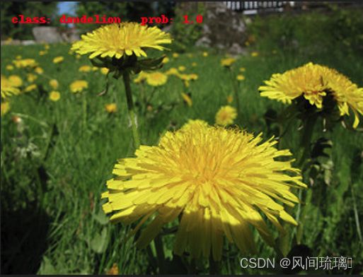
三、实现图像分类

这里使用花朵数据集，下载连接：https://storage.googleapis.com/download.tensorflow.org/example_images/flower_photos.tgz
​

def main():
    device = torch.device("cuda:0" if torch.cuda.is_available() else "cpu")

    # 与训练的预处理一样
    data_transform = transforms.Compose([
        transforms.Resize(256),
        transforms.CenterCrop(224),
        transforms.ToTensor(),
        transforms.Normalize([0.485, 0.456, 0.406], [0.229, 0.224, 0.225])
    ])

    # 加载图片
    img_path = 'dandelion2.jpg'
    assert os.path.exists(img_path), "file: '{}' does not exist.".format(img_path)
    image = Image.open(img_path)

    # image.show()
    # [N, C, H, W]
    img = data_transform(image)
    # 扩展维度
    img = torch.unsqueeze(img, dim=0)

    # 获取标签
    json_path = 'class_indices.json'
    assert os.path.exists(json_path), "file: '{}' does not exist.".format(json_path)
    with open(json_path, 'r') as f:
        # 使用json.load()函数加载JSON文件的内容并将其存储在一个Python字典中
        class_indict = json.load(f)

    # create model
    model = create_model(num_classes=5).to(device)
    # load model weights
    model_weight_path = "./weights/model-60.pth"
    model.load_state_dict(torch.load(model_weight_path, map_location=device))


    model.eval()
    with torch.no_grad():
        # 对输入图像进行预测
        output = torch.squeeze(model(img.to(device))).cpu()
        # 对模型的输出进行 softmax 操作，将输出转换为类别概率
        predict = torch.softmax(output, dim=0)
        # 得到高概率的类别的索引
        predict_cla = torch.argmax(predict).numpy()

    res = "class: {}   prob: {:.3}".format(class_indict[str(predict_cla)], predict[predict_cla].numpy())
    draw = ImageDraw.Draw(image)
    # 文本的左上角位置
    position = (10, 10)
    # fill 指定文本颜色
    draw.text(position, res, fill='red')
    image.show()
    for i in range(len(predict)):
        print("class: {:10}   prob: {:.3}".format(class_indict[str(i)], predict[i].numpy()))


if __name__ == '__main__':
    main()

结束语

感谢阅读吾之文章，今已至此次旅程之终站 。

吾望斯文献能供尔以宝贵之信息与知识也 。

学习者之途，若藏于天际之星辰，吾等皆当努力熠熠生辉，持续前行。

然而，如若斯文献有益于尔，何不以三连为礼？点赞、留言、收藏 - 此等皆以证尔对作者之支持与鼓励也 。