CNN：目标检测Head

一、概述Object Detection

最早深度学习只支持一张图片包含单个目标时，对该图片进行classification或对图片中的单个物体进行classification with localization：

• classification : 适用于一张图片中只有一个目标，以三分类为例 y = [ c1, c2, c3]，直接使用softmax即可；
• classification with localization: 是指在softmax给出分类结果的同时，同时期望给出目标的位置，需添加bounding box的4个参数（bx, by, w, h）, 让网络回归出目标的具体位置，即 y = [pc, bx, by, bh, bw, c1, c2, c3]  

pc的作用：如果包含目标，则pc设为1，再去设定其他参数；如果不是目标，则pc设为0 。这样，对于常见的误检图片（负样本）也可以加入到数据中，降低误检）。

在此基础上，逐渐发展为支持一张图片有多个目标时给出每个目标的类型和位置，即我们现在说的目标检测object detection问题。

object detection: 基于上述classification with localization发展而来的最直观的目标检测算法是滑移窗口+classification算法：在图片内选择窗口，假设是一个窗口内只有一个object的假设，从而将窗口内的问题转化为Classification问题。滑移窗口相当于暴力搜索法，在空间滑移窗口以覆盖不同空间位置，同时，还需要选择不同尺度的窗口以覆盖不同尺度的目标。该方法的缺点是：

• 计算量大，且涉及很多冗余计算；
• 选择的窗口的位置肯定不能保证准确贴合目标位置的，但是也不适合使用滑移窗口+Classification and localization的方法，一方面由于目标有可能不是全部落在窗口中的，另一方面，增加回归bounding box的4个参数会使得计算量更大。

在实际发展中，逐渐发展了很多更简洁、快速、有效的算法。总体而言，根据是否先使用Region Proposal，分为Two-stages和One-stage；根据是否依赖预选框进行正负样本的定义和归一化，分为Anchor based和Anchor free的方法。Anchor based可以是Two stages，也可以是One stage的；Anchor free的方法一般属于One-stage。注意，这些方法中其实出现了3种box，不要混淆它们的概念：

• Anchor box是一些预定义尺寸的box，实质是一些regression reference；
• Region Proposal是基于Anchor box进行了一次Regression获得的class-independent的区域box，随后在该区域提取feature再进行class-dependent的Regression；
• bbox是最终检测结果的框，无论是Anchor based还是Anchor free，无论是Two stages还是One stage，都会产生最终的bbox结果。

在之前的博客中我讲述了CNN网络的Backbone网络的发展历程很大程度地依赖于2010~2017年ImageNet数据集CNN：经典Backbone和Block_yly的博客-CSDN博客 的比赛（主要体现在分类任务），本文讲述的目标检测Head的优化发展更依赖于另一个数据集PASCAL VOC 2005-2012(数据集到2012年就不更新了，但评分网站一直开放，所以到今天为止不断有模型刷榜，算法排名可参见http://host.robots.ox.ac.uk:8080/leaderboard/main_bootstrap.php ）上，本文我们主要使用其中的comp4的进行排名http://host.robots.ox.ac.uk:8080/leaderboard/displaylb_main.php?challengeid=11&compid=4。

二、Two-stages  & Anchor based算法

先利用传统算法或CNN网络给出候选框，再在候选框上运行classification以及进一步回归优化候选框的精确位置。Girshick等人的一些列工作引出了anchor box方法和两阶段模型。

R-CNN （2014，Rich feature hierarchies for accurate object detection and semantic segmentation，VOC2007 mAP=49.6）中，使用三步完成目标检测：

A. 使用传统方法做Region proposals；

B. 将候选框Resize到固定尺寸后放入CNN网络中提取feature，并输出一个固定长度的feature vector；

C. 使用了传统的机器学习方法对提取的feature vector进行分类。

          图片引自Rich feature hierarchies for accurate object detection and semantic segmentation 

这里，只用CNN网络提取特征，对于每一个Region proposal都需要送进一次CNN网络，每张图片对应着~2k个Region proposal，这使得处理一张图片非常慢，无法做到实时；另外，由于最后只是使用了机器学习的方法对之前的Region proposal的候选框做了分类，检测框的定位取决于Region proposal的精度，一般不太不准确。 

在2015年的两篇论文中，先后对步骤C和步骤A进行了优化。

Fast R-CNN （2015，VOC2007 mAP=68.4），论文中针对上述问题，对步骤B和C进行了优化。针对步骤B，这里利用了数据共享，不再是把每一个Region proposal分别送进同一个CNN网络，而是先对整幅图像送入CNN网络提取feature map，随后，把该Region proposal区域投影到feature map，并把提取的feature map的RoI区域送入RoI pooling layer获得到固定尺度的feature map （在2017，Mask R-CNN中改为ROIAlign去除RoI pooling过程中带来的两次量化误差，以获得更准备的预测框位置）；针对步骤C，使用网络的方法代替传统的机器学习，使得网络可以端到端地进行训练，使用Fully connected layers，并在softmax分类的基础上增加了bbox regressor头，使得检测框的定位更加准确。

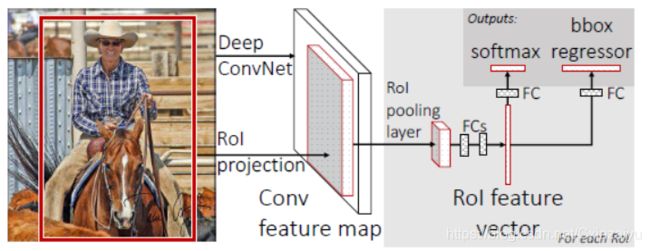
                                                                    图片引自Fast R-CNN

该方法中，Region proposal还是使用传统机器学习方法。

Faster R-CNN （2015, Faster R-CNN: Towards Real-Time Object Detection with Region Proposal Networks，VOC2007 mAP=70.4）中，针对步骤A进行了优化，直接使用CNN网络获得Region proposal，进一步做到Region proposal与提取特征共享计算。即在CNN输出的feature maps基础上加了一个RPN(Region Proposal Network)的头，随后，使用输出的Region proposal进行和上面Fast R-CNN类似的RoI pooling + Classifer(包括softmax分类和bbox regressor)。

  图片引自Faster R-CNN: Towards Real-Time Object Detection with Region Proposal Networks  

其中，RPN网络的结构如下图所示，使用的sliding window是固定尺寸的3x3的feature送入Intermediate layer，reg layer中通过k个不同regressor来来保证分别优化回归k个anchor box。head的参数包括是否包含物体的二分类（2k个参数：属于物体，不属于物体的两分类softmax层；若使用logistic regression则可变为k个参数）和anchor bbox的参数回归获得Region proposals(4k个参数:box中心点的坐标和长宽（x,y,w, h）)。RPN网络中正式提出了使用anchor boxes，anchor boxes是指在每一个3x3的window的feature中回归k个不同尺度和纵横比的boxex的参数（这里在每一个3x3的window中都使用了Anchor boxex，实质是滑移窗口的卷积实现，充分利用GPU的并行计算，并不是依次地进行滑移window）。在原论文中，作者使用了面积为128^2,256^2，512^2三种面积和1:1,2:1, 1:2三种比例分别配对，共9中anchor boxes（即k=9）。

     图片引自Faster R-CNN: Towards Real-Time Object Detection with Region Proposal Networks 

anchor box有两个作用: 

第一，定义正负样本，即建立与标注的目标框真值的关系。

为了让Region Proposal这部分头输出propose的目标框，需要要确定标注的目标框真值与待预测量的对应关系，论文中，是通过anchor box建立和标注目标框真值的关系的，即把标注真值目标框与anchor box进行对应关联。具体实现是把所有与标注真值框有最高IoU的Anchor box以及与标注真值的IoU>0.7的Anchor box都作为positive label, 因此，一个标注真值框可能给多个Anchor box分配positive label。

“For training RPNs, we assign a binary class label (of being an object or not) to each anchor. We assign a positive label to two kinds of anchors: (i) the anchor/anchors with the highest Intersection-overUnion (IoU) overlap with a ground-truth box, or (ii) an anchor that has an IoU overlap higher than 0.7 with any ground-truth box. Note that a single ground-truth box may assign positive labels to multiple anchors. Usually the second condition is sufficient to determine the positive samples; but we still adopt the first condition for the reason that in some rare cases the second condition may find no positive sample. We assign a negative label to a non-positive anchor if its IoU ratio is lower than 0.3 for all ground-truth boxes. Anchors that are neither positive nor negative do not contribute to the training objective”

Anchor与标注真值框之间进行match的代码在Detectron2/detectron2/modeling/matcher.py中的实现如下：

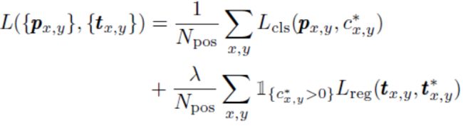
class Matcher(object):
    """
    This class assigns to each predicted "element" (e.g., a box) a ground-truth
    element. Each predicted element will have exactly zero or one matches; each
    ground-truth element may be matched to zero or more predicted elements.

    The matching is determined by the MxN match_quality_matrix, that characterizes
    how well each (ground-truth, prediction)-pair match each other. For example,
    if the elements are boxes, this matrix may contain box intersection-over-union
    overlap values.

    The matcher returns (a) a vector of length N containing the index of the
    ground-truth element m in [0, M) that matches to prediction n in [0, N).
    (b) a vector of length N containing the labels for each prediction.
    """

    def __init__(
        self, thresholds: List[float], labels: List[int], allow_low_quality_matches: bool = False
    ):
        """
        Args:
            thresholds (list): a list of thresholds used to stratify predictions
                into levels.
            labels (list): a list of values to label predictions belonging at
                each level. A label can be one of {-1, 0, 1} signifying
                {ignore, negative class, positive class}, respectively.
            allow_low_quality_matches (bool): if True, produce additional matches
                for predictions with maximum match quality lower than high_threshold.
                See set_low_quality_matches_ for more details.

            For example,
                thresholds = [0.3, 0.5]
                labels = [0, -1, 1]
                All predictions with iou < 0.3 will be marked with 0 and
                thus will be considered as false positives while training.
                All predictions with 0.3 <= iou < 0.5 will be marked with -1 and
                thus will be ignored.
                All predictions with 0.5 <= iou will be marked with 1 and
                thus will be considered as true positives.
        """
        # Add -inf and +inf to first and last position in thresholds
        thresholds = thresholds[:]
        assert thresholds[0] > 0
        thresholds.insert(0, -float("inf"))
        thresholds.append(float("inf"))
        # Currently torchscript does not support all + generator
        assert all([low <= high for (low, high) in zip(thresholds[:-1], thresholds[1:])])
        assert all([l in [-1, 0, 1] for l in labels])
        assert len(labels) == len(thresholds) - 1
        self.thresholds = thresholds
        self.labels = labels
        self.allow_low_quality_matches = allow_low_quality_matches

    def __call__(self, match_quality_matrix):
        """
        Args:
            match_quality_matrix (Tensor[float]): an MxN tensor, containing the
                pairwise quality between M ground-truth elements and N predicted
                elements. All elements must be >= 0 (due to the us of `torch.nonzero`
                for selecting indices in :meth:`set_low_quality_matches_`).

        Returns:
            matches (Tensor[int64]): a vector of length N, where matches[i] is a matched
                ground-truth index in [0, M)
            match_labels (Tensor[int8]): a vector of length N, where pred_labels[i] indicates
                whether a prediction is a true or false positive or ignored
        """
        assert match_quality_matrix.dim() == 2
        if match_quality_matrix.numel() == 0:
            default_matches = match_quality_matrix.new_full(
                (match_quality_matrix.size(1),), 0, dtype=torch.int64
            )
            # When no gt boxes exist, we define IOU = 0 and therefore set labels
            # to `self.labels[0]`, which usually defaults to background class 0
            # To choose to ignore instead, can make labels=[-1,0,-1,1] + set appropriate thresholds
            default_match_labels = match_quality_matrix.new_full(
                (match_quality_matrix.size(1),), self.labels[0], dtype=torch.int8
            )
            return default_matches, default_match_labels

        assert torch.all(match_quality_matrix >= 0)

        # match_quality_matrix is M (gt) x N (predicted)
        # Max over gt elements (dim 0) to find best gt candidate for each prediction
        matched_vals, matches = match_quality_matrix.max(dim=0)

        match_labels = matches.new_full(matches.size(), 1, dtype=torch.int8)

        for (l, low, high) in zip(self.labels, self.thresholds[:-1], self.thresholds[1:]):
            low_high = (matched_vals >= low) & (matched_vals < high)
            match_labels[low_high] = l

        if self.allow_low_quality_matches:
            self.set_low_quality_matches_(match_labels, match_quality_matrix)

        return matches, match_labels

    def set_low_quality_matches_(self, match_labels, match_quality_matrix):
        """
        Produce additional matches for predictions that have only low-quality matches.
        Specifically, for each ground-truth G find the set of predictions that have
        maximum overlap with it (including ties); for each prediction in that set, if
        it is unmatched, then match it to the ground-truth G.

        This function implements the RPN assignment case (i) in Sec. 3.1.2 of
        :paper:`Faster R-CNN`.
        """
        # For each gt, find the prediction with which it has highest quality
        highest_quality_foreach_gt, _ = match_quality_matrix.max(dim=1)
        # Find the highest quality match available, even if it is low, including ties.
        # Note that the matches qualities must be positive due to the use of
        # `torch.nonzero`.
        _, pred_inds_with_highest_quality = nonzero_tuple(
            match_quality_matrix == highest_quality_foreach_gt[:, None]
        )
        # If an anchor was labeled positive only due to a low-quality match
        # with gt_A, but it has larger overlap with gt_B, it's matched index will still be gt_B.
        # This follows the implementation in Detectron, and is found to have no significant impact.
        match_labels[pred_inds_with_highest_quality] = 1

第二，归一化。anchor box的实质对预测量和真值做了归一化，以使得被预测量的范围落在0附近（预测的量变为相对anchor box的offset），而非直接在一个超大的范围直接预测x,y,w,h这些变量，这使得网络可以学习得更准确：

其中，x代表预测量， xa代表anchor box的量，x*代表真值 (y, w, h的角标表示的意义一致)。上面提到会为每一个anchor匹配一个真值框，并分配相应的class label(-1,0,1)分别代表是否是false positive, ignore, true positive)，因此，每个anchor box都是和真值关联的，可以为每个anchor box计算tx*， ty*, tw*, th*；预测时获得tx, ty, tw, th，可以计算loss：

 其中，R代表Loss的函数。

推理时，通过每个anchor预测获得的tx, ty, tw, th在进行解码，获得预测的（x, y, w, h）。

这部分的代码实现可以参见：Detectron2/detectron2/modeling/box_regression.py，使用get_deltas方法获得归一化的回归目标。

class Box2BoxTransform(object):
    """
    The box-to-box transform defined in R-CNN. The transformation is parameterized
    by 4 deltas: (dx, dy, dw, dh). The transformation scales the box's width and height
    by exp(dw), exp(dh) and shifts a box's center by the offset (dx * width, dy * height).
    """

    def __init__(
        self, weights: Tuple[float, float, float, float], scale_clamp: float = _DEFAULT_SCALE_CLAMP
    ):
        """
        Args:
            weights (4-element tuple): Scaling factors that are applied to the
                (dx, dy, dw, dh) deltas. In Fast R-CNN, these were originally set
                such that the deltas have unit variance; now they are treated as
                hyperparameters of the system.
            scale_clamp (float): When predicting deltas, the predicted box scaling
                factors (dw and dh) are clamped such that they are <= scale_clamp.
        """
        self.weights = weights
        self.scale_clamp = scale_clamp

    def get_deltas(self, src_boxes, target_boxes):
        """
        Get box regression transformation deltas (dx, dy, dw, dh) that can be used
        to transform the `src_boxes` into the `target_boxes`. That is, the relation
        ``target_boxes == self.apply_deltas(deltas, src_boxes)`` is true (unless
        any delta is too large and is clamped).

        Args:
            src_boxes (Tensor): source boxes, e.g., object proposals
            target_boxes (Tensor): target of the transformation, e.g., ground-truth
                boxes.
        """
        assert isinstance(src_boxes, torch.Tensor), type(src_boxes)
        assert isinstance(target_boxes, torch.Tensor), type(target_boxes)

        src_widths = src_boxes[:, 2] - src_boxes[:, 0]
        src_heights = src_boxes[:, 3] - src_boxes[:, 1]
        src_ctr_x = src_boxes[:, 0] + 0.5 * src_widths
        src_ctr_y = src_boxes[:, 1] + 0.5 * src_heights

        target_widths = target_boxes[:, 2] - target_boxes[:, 0]
        target_heights = target_boxes[:, 3] - target_boxes[:, 1]
        target_ctr_x = target_boxes[:, 0] + 0.5 * target_widths
        target_ctr_y = target_boxes[:, 1] + 0.5 * target_heights

        wx, wy, ww, wh = self.weights
        dx = wx * (target_ctr_x - src_ctr_x) / src_widths
        dy = wy * (target_ctr_y - src_ctr_y) / src_heights
        dw = ww * torch.log(target_widths / src_widths)
        dh = wh * torch.log(target_heights / src_heights)

        deltas = torch.stack((dx, dy, dw, dh), dim=1)
        assert (src_widths > 0).all().item(), "Input boxes to Box2BoxTransform are not valid!"
        return deltas

    def apply_deltas(self, deltas, boxes):
        """
        Apply transformation `deltas` (dx, dy, dw, dh) to `boxes`.

        Args:
            deltas (Tensor): transformation deltas of shape (N, k*4), where k >= 1.
                deltas[i] represents k potentially different class-specific
                box transformations for the single box boxes[i].
            boxes (Tensor): boxes to transform, of shape (N, 4)
        """
        deltas = deltas.float()  # ensure fp32 for decoding precision
        boxes = boxes.to(deltas.dtype)

        widths = boxes[:, 2] - boxes[:, 0]
        heights = boxes[:, 3] - boxes[:, 1]
        ctr_x = boxes[:, 0] + 0.5 * widths
        ctr_y = boxes[:, 1] + 0.5 * heights

        wx, wy, ww, wh = self.weights
        dx = deltas[:, 0::4] / wx
        dy = deltas[:, 1::4] / wy
        dw = deltas[:, 2::4] / ww
        dh = deltas[:, 3::4] / wh

        # Prevent sending too large values into torch.exp()
        dw = torch.clamp(dw, max=self.scale_clamp)
        dh = torch.clamp(dh, max=self.scale_clamp)

        pred_ctr_x = dx * widths[:, None] + ctr_x[:, None]
        pred_ctr_y = dy * heights[:, None] + ctr_y[:, None]
        pred_w = torch.exp(dw) * widths[:, None]
        pred_h = torch.exp(dh) * heights[:, None]

        x1 = pred_ctr_x - 0.5 * pred_w
        y1 = pred_ctr_y - 0.5 * pred_h
        x2 = pred_ctr_x + 0.5 * pred_w
        y2 = pred_ctr_y + 0.5 * pred_h
        pred_boxes = torch.stack((x1, y1, x2, y2), dim=-1)
        return pred_boxes.reshape(deltas.shape)
def _dense_box_regression_loss(
    anchors: List[Union[Boxes, torch.Tensor]],
    box2box_transform: Box2BoxTransform,
    pred_anchor_deltas: List[torch.Tensor],
    gt_boxes: List[torch.Tensor],
    fg_mask: torch.Tensor,
    box_reg_loss_type="smooth_l1",
    smooth_l1_beta=0.0,
):
    """
    Compute loss for dense multi-level box regression.
    Loss is accumulated over ``fg_mask``.

    Args:
        anchors: #lvl anchor boxes, each is (HixWixA, 4)
        pred_anchor_deltas: #lvl predictions, each is (N, HixWixA, 4)
        gt_boxes: N ground truth boxes, each has shape (R, 4) (R = sum(Hi * Wi * A))
        fg_mask: the foreground boolean mask of shape (N, R) to compute loss on
        box_reg_loss_type (str): Loss type to use. Supported losses: "smooth_l1", "giou",
            "diou", "ciou".
        smooth_l1_beta (float): beta parameter for the smooth L1 regression loss. Default to
            use L1 loss. Only used when `box_reg_loss_type` is "smooth_l1"
    """
    if isinstance(anchors[0], Boxes):
        anchors = type(anchors[0]).cat(anchors).tensor  # (R, 4)
    else:
        anchors = cat(anchors)
    if box_reg_loss_type == "smooth_l1":
        gt_anchor_deltas = [box2box_transform.get_deltas(anchors, k) for k in gt_boxes]
        gt_anchor_deltas = torch.stack(gt_anchor_deltas)  # (N, R, 4)
        loss_box_reg = smooth_l1_loss(
            cat(pred_anchor_deltas, dim=1)[fg_mask],
            gt_anchor_deltas[fg_mask],
            beta=smooth_l1_beta,
            reduction="sum",
        )
    elif box_reg_loss_type == "giou":
        pred_boxes = [
            box2box_transform.apply_deltas(k, anchors) for k in cat(pred_anchor_deltas, dim=1)
        ]
        loss_box_reg = giou_loss(
            torch.stack(pred_boxes)[fg_mask], torch.stack(gt_boxes)[fg_mask], reduction="sum"
        )
    elif box_reg_loss_type == "diou":
        pred_boxes = [
            box2box_transform.apply_deltas(k, anchors) for k in cat(pred_anchor_deltas, dim=1)
        ]
        loss_box_reg = diou_loss(
            torch.stack(pred_boxes)[fg_mask], torch.stack(gt_boxes)[fg_mask], reduction="sum"
        )
    elif box_reg_loss_type == "ciou":
        pred_boxes = [
            box2box_transform.apply_deltas(k, anchors) for k in cat(pred_anchor_deltas, dim=1)
        ]
        loss_box_reg = ciou_loss(
            torch.stack(pred_boxes)[fg_mask], torch.stack(gt_boxes)[fg_mask], reduction="sum"
        )
    else:
        raise ValueError(f"Invalid dense box regression loss type '{box_reg_loss_type}'")
    return loss_box_reg

随后，获得预测值后再解码成box ( Detectron2/detectron2/modeling/proposal_generator/rpn.py)

    def _decode_proposals(self, anchors: List[Boxes], pred_anchor_deltas: List[torch.Tensor]):
        """
        Transform anchors into proposals by applying the predicted anchor deltas.

        Returns:
            proposals (list[Tensor]): A list of L tensors. Tensor i has shape
                (N, Hi*Wi*A, B)
        """
        N = pred_anchor_deltas[0].shape[0]
        proposals = []
        # For each feature map
        for anchors_i, pred_anchor_deltas_i in zip(anchors, pred_anchor_deltas):
            B = anchors_i.tensor.size(1)
            pred_anchor_deltas_i = pred_anchor_deltas_i.reshape(-1, B)
            # Expand anchors to shape (N*Hi*Wi*A, B)
            anchors_i = anchors_i.tensor.unsqueeze(0).expand(N, -1, -1).reshape(-1, B)
            proposals_i = self.box2box_transform.apply_deltas(pred_anchor_deltas_i, anchors_i)
            # Append feature map proposals with shape (N, Hi*Wi*A, B)
            proposals.append(proposals_i.view(N, -1, B))
        return proposals

         这是经典的两阶段的网络，因为图片中可能包含多个目标，先通过Region proposal获得一些框（大概率使得每个框内最多包含一个物体），再基于这些propose的框使用Classification and localization的方法进行分类和回归，这种方法在目标检测发展初期的知识框架中是非常直观的。先进行Region proposal（此时已经进行了一次box的回归，通过回归anchor boxes获得proposals），步骤C与Fast R-CNN相同，再基于proposals的框内提取的feature进行bbox的第二次回归，理论上,由于region proposal的区域的feature更贴近物体的特征，基于此特征再送入网络回归的bbox应该相对于单阶段的方法更准确。

        这个网络的缺点是训练过程复杂，由于Fast R-CNN训练时是假定给定了proposal，如果同时训练proposal和Fast R-CNN会很难收敛，所以，作者先训练RPN，随后，使用训练好的RPN给出的proposal训练Fast R-CNN部分，这里基础的CNN部分还没有进行计算共享。接下来，使用Fast R-CNN部分训练好的参数初始化RPN部分，并固定相同的CNN层，单独更新RPN特有的层。最后，在固定相同的CNN层，优化Fast R-CNN独有的层。

三、One-stage detector

一般的对单阶段检测模型的分类的说法是anchor-based的和anchor-free的，早期是anchor-based，现在主要是anchor-free的。但是，回看论文发展的过程，其实并不是这样，因为最早期的单阶段模型Densebox和YOLO的第一版就是没有anchor的概念的，而是创新地使用一个channel代表物体是否存在object confidence score，其他channel代表bbox的其他物理量，通过object confidence score的channel的空间位置确定与标注真值的关系（也是目前主流使用的方法，代替了上面提到的anchor box的第一个作用确定与真值的对应关系）；后来SSD等论文中引入了Faster R-CNN中anchor bbox的概念是为了在FPN上确定正负样本的定义，并使用到了上面提到的anchor box的第二个作用（归一化）来提升精度；再到现在发现使用基于概率表示目标是否存在的方法更有效，才又变为anchor-free。

可以说，在单阶段模型中，anchor box是目标检测发展中间过程引入的提升目标角检测精度的trick之一，但以anchor是否存在来划分目标检测的发展是容易让人引起误解的。看CNN把一个任务formulate成什么问题主要是看设计loss function时是如何构建标注真值与预测值的对应关系的（即how to define positive and negative training samples）。因此，如果一定要划分的话，其实存在一个更好地划分方法：根据object confidence score的feature map是0-1还是概率值划分。

1. 真值0 or 1的object confidence score

Densebox（2015，Densebox: Unifying landmark localization with end to end object detection）使用全卷积神经网络，去除了全连接层，使用输出的不同channel分别代表不同的预测的物理量。Densebox输入分辨率为mxn的图像，输出为m/4xn/4x5的channel，5个channel分别预测object confidence score（该位置是否存在目标）+ bbox的位置（feature的每个位置到目标框的左上角坐标（xt,yt）和右下角坐标（xb,yb）的距离）。相当于原图mxn的分辨率上每4x4的像素就propose一个目标框，最后对于object confidence score超过阈值的目标框使用NMS去除重叠。

其中，training过程设定5个channel的真值时，object confidence socre选取目标框中心为圆心，半径为目标框尺寸的0.3倍之内的圆形设为1，其余位置设为0；相应地，其他表示bbox的位置的4个channel仅在object confidence score设为1的圆内的区域内设定目标框到该像素的位置差。

为了增大感受野，论文先将mxn的输入卷积到较小的feature map后，再通过upsample到m/4xn/4的分辨率。

这是黄李超大神非常经典的论文，这篇文章中包含很多好的思想：

使用全卷积神经网络，在output每个channel上表示一个物理量，为每个resolution预测一个bbox。把这种思想稍微扩展下，为output channel的每个resolution预测一个类别，每个channel代表一类，就是的经典语义分割的论文（2015，Fully Convolutional Networks for Semantic Segmentation）。

YOLO (2016，You Only Look Once: Unified, Real-Time Object Detection，VOC2007 mAP=57.9），为了解决Faster-CNN系列的Two stages方法训练复杂、推理较慢的问题，Girshick又参与了One-stage的方法的YOLO工作。在卷积层尺寸为S*S的feature map上的每一个cell上直接回归一个或多个bounding box。

YOLO中把输出层的分辨率大大降低到7x7，这么小的分辨率就无法像上面Densebox那样把output feature在目标框内一个区域范围中的resolution都设为存在目标的ground truth，因为YOLO输出的分辨率上可能1个grid上面就包含多个物体了，也可能一个物体横跨多个grid。设计loss function时，为了建立标注真值与预测值的对应关系，将YOLO原图也与feature map对应地划分成S*S的grid cell，并将标注真值框中心点所在原图的grid cell所对应位置的feature map中的小cell的box分配positive label 。即feature map中只有一个cell中的一个box负责预测一个真值框。【注意：这里将原图换分成S*S个网格仅仅是为了建立标注框真值与feature map中预测的box的对应关系，以建立loss function。（这种建立真值与预测框的对应关系的方法是直观的，但不是唯一的，比如，如果做loss时保持让feature map中的左上的grid cell的bounding box向量对应原图中右下角的grid cell标注的bounding box，那么在推理时也是能给出正确的预测结果的，只需要保持原图分割的大grid cell与feature map中的小grid cell对应关系始终一致即可。）不要误解成原图中的大grid cell进行卷积直接卷积缩小到了feature map中的小cell ，这是看YOLO论文时直观上看示意图最容易造成误解的地方，因为最后的feanture map之前是两个全连接层，所以预测每一个bbox的时候都是使用了整幅图像的feature （注意区分：在Faster R-CNN中的RPN是放入3x3的window的局部feature；获得Region proposal后再使用对应的区域feature放入detector头进行回归），网络中使用了全连接层，feature map中每一个小grid cell对应的感受野是整幅原图。】

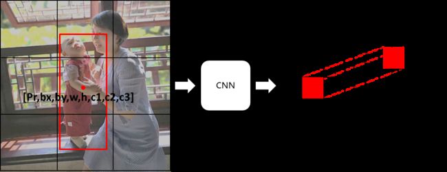
                                            原图bounding box与feature map中tensor对应关系示意

先以在S*S的feature map上的每一个cell上回归一个bounding box为例。设计CNN网络最后一层的feature map为S*S*length[ y' ]的tensor，每个feature map中的小cell的结果为y'=[Pr, bx, by, w, h, c1, c2, c3]，如上图所示。其中，Pr表示confidence，该confidence的定义是Pr(object)*IoU_gt&pred，反应了该box包含目标以及预测的框准确性的概率，每个框对应一个Pr；c1~c3表示的是conditional class 类别的概率Pr(Classi|Object)，每个cell对应一组Pr(Classi|Object)，有多少类别就使用多少channel，定义为属于相应类别真值就设为1，否则就设为0。这里的Pr相当于Faster-RCNN中RPN阶段的objectness score，c1~cn的conditional class相当于Faster-RCNN中第二阶段的分类【可能是都有Ross Girshick参与的原因吧，YOLO这个objectness score和class class-specific confidence的设计很像是把Faster-RCNN压在了一个一阶段】。注意，这里的方法非常巧妙，训练时在不同channel上同时预测objectness score和conditional class probabilities（只有在存在物体时才会有该部分loss），预测时最终计算每个框的最终的class-specific confidence scores把两者结合起来，class-specific confidence scores=Pr(Classi|Object) * Pr(object)*IoU_gt&pred。

另外，（bx,by）为bounding box的中心点在原图grid cell中的相对位置（偏移量offset），（w,h）是相对于整幅图像的长宽（图像归一化后，w和h都在0~1之间），bounding box的长和宽可以超过grid cell大小（因为预测每一个bbox的时候都是使用了整幅图像的feature）。

• 标注：每个真实目标仅标注了一个框；
• 训练：训练loss时将目标框分配给其中心点落在的grid cell中，把原图标注的bounding box所对应的参数y=[Pr, bx, by, w, h, c1, c2, c3]与该bounding box的中心点所落在的大grid cell的空间位置相对应的的feature map中小grid cell的上的向量 y^ = [Pr, bx, by, w, h, c1, c2, c3]求loss。
• 推理：每一个grid cell都会propose一个bounding box，当一个目标覆盖多个grid cell时，可能被多个grid cell都propose出；最后，对于IOU超过一定阈值的候选框通过NMS进行过滤，仅保留可能性最大的。

以上方法另每个feature map的cell中预测了一组y=[Pr, bx, by, w, h, c1, c2, c3]与原图大grid cell中所负责的bounding box对应。但考虑到输出的分辨率7x7非常小，肯定会出现多个目标的中心点都落在同一个大的grid cell的情况，这时如何处理？论文中也提到可以让每个cell中预测多个box，以每个cell预测两个目标框为例讲解在cell中propose多个bounding box的方法：y' = [ Pr1, bx1, bx2, w1, h1, c11, c12, c13, Pr2, bx2, by2, w2, h2, c21,c22, c23]），对应地，在最后一层feature map上增加channel代表新增加的[Pr2, bx2, by2, w2, h2, c21,c22, c23]即可。这样就可以覆盖两个目标框中心点落在一个原图大grid cell中的情况。为了覆盖更复杂的重叠情况可以在每个feature map中覆盖更多组bounding box参数，方法与两个box的方法相同。在设计loss function时应该让真值框与第几个box对应呐？标注真值目标框中心点落在哪个grid cell是固定的，当grid cell对应可以预测多个框时，目标真值框与grid cell中具体哪个框对应不是预设的（这里和Anchor box提前根据IoU预设好与目标框的对应关系不同），而是随机初始化后predict的box与真值目标框的IoU较高的box分配positive lable，这产生的结果是随着训练按照预定顺序的每个框更适合预测某一尺寸、长宽比的目标（开始一点点差别导致后来不同的分工）。

YOLO缺点：相比于Faster R-CNN等Two Stages模型，YOLO预测的bounding box的框（中心点以及长宽）不够精确，VOC2007 mAP仅为63.4。其背后的原因如下：

• Two Stages方法中进行了两次Anchor box的回归，并且在第二次回归时使用第一次回归给出的更准确的feature作为输入；而One Stage方法中把全图特征作为输入，且只进行一次回归，输入给回归的特征选择肯定不像Two Stages选取的特征那样准确和精细。
• a. YOLO中只让一个feature map中的cell对应bounding box的真值（即bounding box中心点对应的cell），然而，实际上一个bounding box可能跨越很多cell，这些cell和bounding box的标注真值也是关联的，但YOLO中loss function的设计忽略了这些关联，可能也会造成网络训练不易收敛、预测效果不好。
• b. YOLO使用的feature map是经过严重downsample的7x7的，且每个cell只使用了2个Anchor box，使得对多尺度处理水平不强。（Faster R-CNN中RPN使用的是WxH=~2400，会提供更多Anchor box，所以论文中说其很好地处理了多尺度）。

在以上问题中，第一个问题是One Stage相对于Two Stages方案固有的缺陷；问题a和问题b是可以快速改进的。

SSD（2016，SSD: Single Shot MultiBox Detector，VOC2007 mAP=75.8）针对上述YOLO的两个问题做了改进：

• a.引入上面两阶段模型Faster R-CNN中的anchor box的概念，以及相应anchor box归一化计算bbox中心点和长宽的方法，可以让预测更精准。同时，不让bounding box真值仅关联其中心点对应的feature map中的cell，凡是anchor box与bounding box标注真值之间的jaccard overlap>0.5的anchor box都参与标注真值求loss。
• b. 在不同尺度的多个feature map中预测bounding box（每一层feature map预测的向量直接与对应的原图划分的grid cell对应的bounding box的真值建立对应关系），这样训练出的模型会让不同尺度的feature map更适合准确预测出相应尺度的bounding box。

采用以上两个措施使得训练更易收敛，预测bounding box的结果更加准确。

 YOLO2（2017，YOLO9000: better, faster, stronger，VOC2007 mAP=75.4）中对YOLO做了trick的探索和性能改进，具体工作如下：

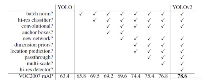
注意：YOLO2表格和文章中有一个容易引起理解歧义的地方，是anchor boxes一行显示使用anchor boxes反而使得mAP从69.5降低到69.2，这里并不是指anchor boxes的思想不对，而是直接按照Faster R-CNN的论文中的像素面积和比列匹配的anchor boxes的尺度和比例在YOLO上表现不好，作者使用的是dimension priors，即把数据集的目标进行聚类，得到了5个dimension priors，并使用下图的公式预测tx, ty, tw, th量。其思想的实质就是anchor boxes, 只是实现的细节与 Faster R-CNN不同，所以表格中说明没有使用anchor boxes其实是没有按照Faster R-CNN那样使用anchor boxes而已。

下图在求bx和by中心点位置上，求取的是在小格内的偏移量tx和ty，相比于直接回归中心点bx和by，预测tx和ty是较小量，更容易预测准；求bw和bh的公式中，pw和ph为anchor boxes的宽和长，把求取bw和bh转化成了tw和th，当tw和th为0时，bw=pw，bh=ph，因为，回归tw和th也是在anchor boxes附近预测接近0的量，更加准确。相对于YOLO最初的工作直接回归bbox的中心点的位置bx、by & bbox的长度bw和宽度bh，mAP显著提升了将近5个百分点（如上表所示），其实这就是anchor boxes的核心思想：引入anchor box把被预测量归一化，让网络预测绝对值比较小的量。

在Anchor based方法中，为了有效预测出结果，使用了大量的Anchor box，实际上获得的positive label要远少于negative label，造成class imbalance,Tsung-Yi Lin等人意识到这是One Stage精度提升的主要瓶颈之一，并在 Focal Loss for Dense Object Detection （2017）论文中提出了新的focal loss来解决class imbalance的问题，并展示了使用Focal Loss在One Stage的方法上超过Two Stage准确度的。

2. 真值概率图的object confidence score （即heatmap）

在上面0-1的object confidence score方法中，确立标注真值与预测值的对应关系时，无论是否使用anchor box，总归需要忽略掉部分与标注真值目标框有关系的预测值（IoU低于阈值的）：YOLO中每个标注真值bounding box仅分配给其中心点对应的feature map的cell中；SSD根据anchor box和标注真值bounding box的overlap设定阈值，让overlap大于阈值的anchor box都与bounding box对应计算loss。以上两种将anchor box与标注真值bounding box建立对应关系的方法都忽略了很多与标注真值bounding box关联的候选框，使得训练也不易收敛或预测效果不好。引入概率图后object confidence score，在真值处设置Gaussian函数，让真值周边的resolution也与真值关联，但是这种关联随着距离真值越远而逐渐降低。

CornerNet （2018, CornerNet: Detecting Objects as Paired Keypoints）受到keypoints关键点检测方法的启发，使用heatmap表示目标bbox的角点存在的概率。在训练时，表示object confidence score的真值heatmap是在标注目标框中心利用unnormalized 2D Gaussian表示存在角点的概率真值y。设计loss function中，并不是平等地惩罚negative label，而是随着距离positive label增大而增加惩罚。 则loss function中使用（1-y）项即可表示随着距离真值增加而增加惩罚。论文中使用C个channel的heatmap，其中，C是分类的数量。在预测时，取heatmap中的极大值（需要增加一些阈值）作为角点存在的位置。

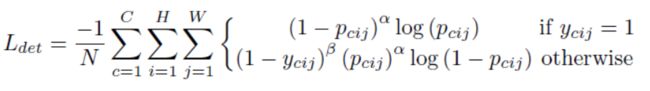
同时，由于输出的feature map的resolution降低了，左上和右下两个角点各自使用一个channel表示角点的offset，通过回归offset的通道计算降采样前的位置，这点在其他channel回归offset是与YOLO类似的。训练时，仅取标注真值位置对应的offset channel的预测值与标注真值求loss function；预测时，取heatmap中的极大值对应位置的offset channel的值来decode角点的精确位置。

从上面两个公式可以看出，求object confidence score时是对全heatmap每个像素进行积分，求offset仅针对真值对应的位置的loss进行求和。 

备注：由于在CornerNet中使用两组heatmap分别预测目标的左上和右下角点，为了确定目标bbox，需要确定哪个左上角点和右下角点是一组，CornerNet中针对每个corner预测一组embedding vector（embedding vector可以理解成以前的点和描述子），embedding vector相近的两个corner组成一个bounding box的两个角点。另外，针对目标检测的corner实际往往落在目标之外，不能直接用局部特征确定corner的问题，使用corner pooling，在CNN输出的feature map后加上corner pooling层，随后基于corner pooling后的feature map再获得最终的feature map（包含了heatmap, offset，embedding）。

CenterNet (2019，CenterNet: Keypoint Triplets for Object Detection)针对CornerNet带来一些虚检框的问题增加了中心点条件进行过滤：在CornerNet预测corner获得bbox的基础上，另外增加一组Heatmap预测目标的中心点，必须在预测的bbox的中心区域中同时包含该Heatmap给出的中心点时才保留该bbox，否则去除该bbox。

上面的Anchor Free的方法中面临着一个问题，就是要组合corner，以形成bbox，后处理较复杂。

CenterNet （2019，Objects as Points）论文中（非常有趣的是，Xingyi Zhou等人在该文章中的方法也起名为CenterNet，和上面一篇文章的网络重名了！），选取标注框的中心点作为真值，同样根据与中心点距离分配reduced negative loss，使用heatmap表示中心点存在的概率。为每一个类别分配一个heatmap，如果是C个类别就有C个heatmap的channel （注意：这里和YOLO不同，不是一个channel负责objectness score判断是否存在物体+C个channel判断C个类别，centernet中直接使用C个channel判断每个类别存在与否和所属的响应的类别概率classification）。与YOLO系列一个表示物体存在概率的channel （confidence）+ C个表示不同类别的channel不同，这里直接把两个概念合并了，heatmap表示的就是某一类物体存在的概率。

同样，保留中心点offset以再将分辨率的output channel上还原中心点位置。目标框的长、宽全部作为feature map中的channel直接回归得到。 具体的操作方法和offset类似（训练时，标注真值位置对应的表示长的channel、宽的channel的预测值与对应的标注真值求loss function；预测时，取heatmap中的极大值对应位置的长宽channel的值来decode角点的精确位置。）目标框的位置可以由如下公式恢复（中心点所在的grid，预测的中心点的offst，预测bbox的长宽）：

另外，使用该框架还可以回归其他物理量，比如，针对3D-OD的任务，还可以拓展channel表示相机坐标系下目标的depth等，只需要能获取该属性的真值，为属性增加channel即可，如下图所示。

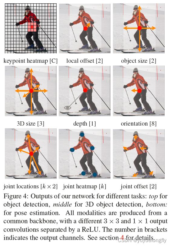
 使用基于heatmap的方法后，论文中output channel的stride选取为4，不像YOLO那样把分辨率降低到7x7或13x13那么小。

Anchor free方法的核心是引入heatmap方法确定物体是否在某处存在，相比于anchor的方法更好地关联了真值和预测量。

缺点是对bbox的长和宽通道的预测上，没法再归一化成小量，可能使得长和宽预测不准，为了解决这个问题，引入IoU loss?

在该centernet方法中，classification score的channel上的正样本的定义可以在整个目标框的范围，也可以选择根据目标框尺寸选择一定中心区域分配成正样本，但是，在预测offset和bbox尺寸的channel上，都只是针对目标框中心点对应的位置作为正样本预测的（也没法让每一个框内的classification score位置都回归目标同样的w,h），即只通过标注真值中心点位置的预测量和真值计算loss function。也就是没有解决其他regression量的正负样本定义的问题。这会带来一个问题，如果classifcation score对应位置有偏差，那么取其他channel相位位置的物理量偏差就很大（因为这些位置的值是没有显式参与到loss function优化的）。

FCOS （2019，FCOS: Fully Convolutional One-Stage Object Detection）同样直接使用C个channel的heatmap表示classfication，和centernet不同的是，针对上面centernet回归目标的w,h时只能针对目标框中心点所在位置回归的问题，转为回归每个点到目标框上下左右的距离t、b、l、r，如下图所示，这样，在回归目标框位置时，也可以针对标注的真值框内的每个grid的正样本都回归目标框的位置，稠密地预测标注真值框内每个grid位置到目标框上下左右四个边的距离，从而保证所有关联到bounding box的grid都参与到与标注真值bounding box求loss，而不是仅在目标框中心点回归其他物理量。

对于回归的积分也是在整个x,y平面做的：

为了在推理时过滤掉目标边缘regress出的低质量的bbox分支，在训练时迭代一个centerness的分支（表示距离中心点距离），在推理时，由该分支的结果与目标object score的channel相乘后，根据该结果对目标框做nms。

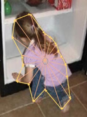
Polarmask（2019，Polarmask: Single shot instance segmentation with polar representation）使用类似FCOS方法，回归多个距离，用检测的方法实现实例分割。如下图所示：

四、Combined one-stage and two-stage

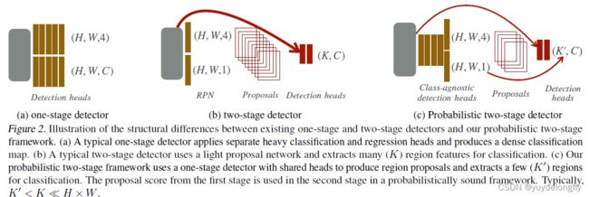
       Probabilistic two-stage detection(2021)使用one stage detector作为RPN模型，但第一阶段比经典的one stage设置的轻，但比经典的two-stage中的第一阶段重；这样，保证有更少的更高质量的候选框进入第二阶段，使得第二阶段的计算量比经典的两阶段中的第二阶段总体的计算量小。使得该方法比经典的one-stage和two-stage都快。

五、应用

以上论文中给出了通用的算法，针对具体的任务，需要根据任务的特点调整网络。

参见：CNN：目标检测在自动驾驶应用中的应用_yuyuelongfly的博客-CSDN博客