【Hydro】水文模型比较框架MARRMoT - 包含47个概念水文模型的Matlab代码

说明

MARRMoT是一个新的水文模型比较框架，允许不同概念水文模型结构之间的客观比较。该框架为47个独特的模型结构提供了Matlab代码，所有模型结构的标准化参数范围以及每个模型的强大数值实现。该框架提供了大量的文档，用户手册和几个工作流脚本，给予如何使用该框架的例子。包括以下模型：

• FLEX-Topo
• IHACRES
• GR4J
• TOPMODEL
• SIMHYD
• VIC
• LASCAM
• TCM
• TANK
• XINANJIANG
• HYMOD
• SACRAMENTO
• MODHYDROLOG
• HBV-96
• MCRM
• SMAR
• NAM
• HYCYMODEL
• GSM-SOCONT
• ECHO
• PRMS
• CLASSIC
• IHM19

MARRMoT框架中的模型期望接近它们所基于的原始模型，但差异是不可避免的。在许多情况下，一个模型存在多个版本，但这些版本并不总是很容易区分的。存在一定程度的模型名称相等性，其中单个名称用来指代同一基模型的各种不同版本。一个很好的例子是TOPMODEL，其中许多变体存在于基于地形指数的最初概念之上。MARRMoT模型往往基于任何给定模型的旧出版物，而不是新出版物（以接近原作者的“预期”模型），但我们的选择是务实的，以实现MARRMoT中可用通量和模型结构的更大多样性。每个模型的描述列出了构成该模型MARRMoT版本基础的论文。

MARRMoT框架以模块化的方式设置，并以单个的通量文件作为基本的构建块。模型文件通过指定每个模型的内部工作方式来为其定义一类对象，而超类文件则定义了所有模型通用的所有过程。图1显示了工具箱结构的示意图概述。

源代码

降雨径流模型的模块化评估

运行实例

workflow_example_1.m

这个示例工作流程包含一个单一模型对单一集水区的应用示例。它包括5个步骤：

1. 数据准备
2. 模型选择和设置(设置参数)
3. 模型求解器设置
4. 模型生成和设置
5. 模型运行
6. 输出可视化
   

workflow_example_2.m

这个示例工作流程包含一个单一模型对单一集水区的应用示例。它包括5个步骤：

1. 数据准备
2. 模型选择和设置(默认参数)
3. 模型求解器设置
4. 模型生成和设置
5. 模型运行
6. 输出可视化
   

workflow_example_3.m

这个示例工作流程包含多个模型对单一集水区的应用示例。它包括6个步骤：

1. 数据准备
2. 模型选择和设置
3. 模型求解器设置
   对于列表中的每个模型：
   5. 模型生成和设置
   6. 模型运行
   7. 输出可视化
   

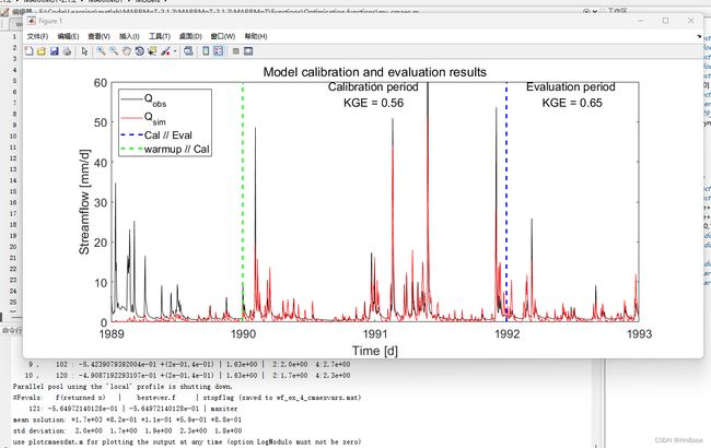
workflow_example_4.m

这个示例工作流程包含了一个单一模型对单一集水区的校准应用示例。它包括7个步骤：

1. 数据准备
2. 模型选择和设置
3. 模型求解器设置和时间步进方案
4. 校准设置
5. 模型校准
6. 校准结果评估
7. 输出可视化

优化方法采用的是CMA-ES算法，算法迭代10次结果

测试

原始代码根据作者描述，在MATLAB版本9.11.0.1873467（R2021b）上开发的，并使用Octave 6.4.0进行了测试。笔者使用R2017a时，出现了几个可能是兼容性的问题。

1、 结构体兼容性问题

动态字段或属性名称必须为字符矢量。

将string转换为char，即可使用结构体动态赋值。

2、append的兼容性问题

错误使用 append (line 38)
Wrong number of input arguments for obsolete matrix-based syntax.

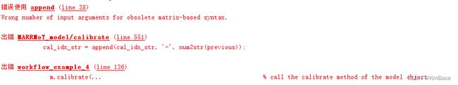
在MATLAB中，append函数是用来将矩阵或数组的元素添加到另一个矩阵或数组的末尾。如果你想将字符串连接到另一个字符串，可以使用cat函数或者简单的加号+。

3、参数优化时间过长的问题

CMA-ES算法终止的参数，可以根据需要修改示例中的条件，比如调小MaxIter。

还修改优化文件my_cmaes.m，显示更多迭代过程

4、修改后的MARRMoT_model.m

classdef MARRMoT_model < handle
% Superclass for all MARRMoT models
    
% Copyright (C) 2019, 2021 Wouter J.M. Knoben, Luca Trotter
% This file is part of the Modular Assessment of Rainfall-Runoff Models
% Toolbox (MARRMoT).
% MARRMoT is a free software (GNU GPL v3) and distributed WITHOUT ANY
% WARRANTY. See  for details.

    properties
        % attribute to store whether we are running MATLAB or Octave
        isOctave          % 1 if we're on Octave, 0 if MATLAB
        % static attributes, set for each models in the model definition
        numStores         % number of model stores
        numFluxes         % number of model fluxes
        numParams         % number of model parameters
        parRanges         % default parameter ranges
        JacobPattern      % pattern of the Jacobian matrix of model store ODEs
        StoreNames        % Names for the stores
        FluxNames         % Names for the fluxes
        FluxGroups        % Grouping of fluxes (useful for water balance and output)
        StoreSigns        % Signs to give to stores (-1 is a deficit store), assumes all 1 if not given
        % attributes set at the beginning of the simulation
            % directly by the user
        theta             % Set of parameters
        delta_t           % time step
        S0                % initial store values
        input_climate     % vector of input climate
        solver_opts       % options for numerical solving of ODEs
            % automatically, based on parameter set
        store_min         % store minimum values
        store_max         % store maximum values
        % attributes created and updated automatically throughout a
        % simulation
        t                 % current timestep
        fluxes            % vector of all fluxes
        stores            % vector of all stores
        uhs               % unit hydrographs and still-to-flow fluxes
        solver_data       % step-by-step info of solver used and residuals
        status            % 0 = model created, 1 = simulation ended

    end
    methods
        % This will run as soon as any model object is created
        function [obj] = MARRMoT_model()
            obj.isOctave = exist('OCTAVE_VERSION', 'builtin')~=0;
            % if running in Octave, load the optim package
            if obj.isOctave; pkg load optim; end
        end
        function [] = set.isOctave(obj, value); obj.isOctave = value; end
        
        % Set methods with checks on inputs for attributes set by the user:
        function [] = set.delta_t(obj, value)
            if numel(value) == 1 || isempty(value)
                obj.delta_t = value;
                obj.reset();
            else
                error('delta_t must be a scalar')
            end
        end
        function [] = set.theta(obj, value)
            if numel(value) == obj.numParams || isempty(value)
                obj.theta = value(:);
                obj.reset();
            else
                error(['theta must have ' int2str(obj.numParams) ' elements'])
            end
        end
        function [] = set.input_climate(obj, value)
            if isstruct(value)
                if isfield(value, 'delta_t')
                    obj.delta_t = value.delta_t;
                elseif isempty(obj.delta_t)
                    error(['delta_t is not in input climate struct: '...
                           'add it with obj.delta_t = delta_t'])
                end
                if isfield(value, {'precip' 'pet' 'temp'})
                    P = value.precip/obj.delta_t;
                    Ea = value.pet/obj.delta_t;
                    T = value.temp/obj.delta_t;
                    obj.input_climate = [P(:) Ea(:) T(:)];
                    obj.reset();
                else
                    error(['Input climate struct must contain fields: '...
                           'precip, pet, temp']);
                end
            elseif isnumeric(value)
                if size(value,2)  || isempty(value)
                    obj.input_climate = value;
                    obj.reset();
                else
                    error(['Input climate must have 3 columns: '...
                           'precip, pet, temp']);
                end
            else
                error(['Input climate must either be a struct or '...
                       'a numeric array of 3 columns']);
            end
        end
        function [] = set.S0(obj, value)
            if numel(value) == obj.numStores || isempty(value)
                obj.S0 = value(:);
                obj.reset();
            else
                error(['S0 must have ' int2str(obj.numStores) ' elements'])
            end
        end
        function [] = set.solver_opts(obj, value)
            % add options to default ones
            obj.solver_opts = obj.add_to_def_opts(value);
            obj.reset();
        end
        
        % INIT_ runs before each model run to initialise store limits,
        % auxiliary parameters etc. it calls INIT which is model specific
        function obj = init_(obj)
            % min and max of stores
            obj.store_min = zeros(obj.numStores,1);
            obj.store_max = inf(obj.numStores,1);
            
            % empty vectors of fluxes and stores
            t_end = size(obj.input_climate, 1);
            obj.stores = zeros(t_end, obj.numStores);
            obj.fluxes = zeros(t_end, obj.numFluxes);
            
            % empty struct with the solver data
            obj.solver_data.resnorm   = zeros(t_end,1);
            obj.solver_data.solver = zeros(t_end,1);
            if(~obj.isOctave); obj.solver_data.solver = categorical(obj.solver_data.solver); end;
            obj.solver_data.iter   = zeros(t_end,1);
            
            % model specific initialisation
            obj.init();
        end
        
        % RESET is called any time that a user-specified input is changed
        % (t, delta_t, input_climate, S0, solver_options) and resets any
        % previous simulation ran on the object.
        % This is to prevent human error in analysing results.
        function obj = reset(obj)
        	obj.t = [];                 % current timestep
            obj.fluxes = [];            % vector of all fluxes
            obj.stores = [];            % vector of all stores
            obj.uhs = [];               % unit hydrographs and still-to-flow fluxes
            obj.solver_data = [];       % step-by-step info of solver used and residuals
            obj.status = 0;             % 0 = model created, 1 = simulation ended
        end
        
        % ODE approximation with Implicit Euler time-stepping scheme
        function err = ODE_approx_IE(obj, S)
            S = S(:);
            delta_S = obj.model_fun(S);
            if obj.t == 1; Sold = obj.S0(:);
            else; Sold = obj.stores(obj.t-1,:)';
            end
            err = (S - Sold)/obj.delta_t - delta_S';
        end 
        
        % SOLVE_STORES solves the stores ODEs 
        function [Snew, resnorm, solver, iter] = solve_stores(obj, Sold)
            
            solver_opts = obj.solver_opts;
            
            % This reduces the tolerance to a fraction of the smallest store,
            % if stores are very small, with 1E-6 as minimum
            % (if resnorm_tolerance is 0.1 as default)
            resnorm_tolerance = solver_opts.resnorm_tolerance * min(min(abs(Sold)) + 1E-5, 1);
            
            % create vectors for each of the three solutions (NewtonRaphon,
            % fsolve and lsqnonlin), this way if all three run it takes the
            % best at the end and not the last one.
            Snew_v    = zeros(3, obj.numStores);
            resnorm_v = Inf(3, 1);
            iter_v    = ones(3,1);
            
            % first try to solve the ODEs using NewtonRaphson
            if(~obj.isOctave) %if MATLAB
                [tmp_Snew, tmp_fval] = ...
                            NewtonRaphson(@obj.ODE_approx_IE,...
                                          Sold,...
                                          solver_opts.NewtonRaphson);
            else              % if Octave
                [tmp_Snew, tmp_fval] = ...
                            NewtonRaphson_octave(@obj.ODE_approx_IE,...
                                                 Sold,...
                                                 solver_opts.NewtonRaphson);
            end
            tmp_resnorm = sum(tmp_fval.^2);
            
            Snew_v(1,:)  = tmp_Snew;
            resnorm_v(1) = tmp_resnorm;
            
            % if NewtonRaphson doesn't find a good enough solution, run FSOLVE
            if tmp_resnorm > resnorm_tolerance  
                [tmp_Snew,tmp_fval,~,tmp_iter] = ...
                            obj.rerunSolver('fsolve', ...              
                                            tmp_Snew, ...                  % recent estimates
                                            Sold);                         % storages at previous time step
                
                tmp_resnorm = sum(tmp_fval.^2);
                
                Snew_v(2,:)  = tmp_Snew;
                resnorm_v(2) = tmp_resnorm;
                iter_v(2)    = tmp_iter;

                % if FSOLVE doesn't find a good enough solution, run LSQNONLIN
                if tmp_resnorm > resnorm_tolerance
                    [tmp_Snew,tmp_fval,~,tmp_iter] = ...
                            obj.rerunSolver('lsqnonlin', ...              
                                            tmp_Snew, ...                  % recent estimates
                                            Sold);                         % storages at previous time step
                    
                    tmp_resnorm = sum(tmp_fval.^2);

                    Snew_v(3,:)  = tmp_Snew;
                    resnorm_v(3) = tmp_resnorm;
                    iter_v(3)    = tmp_iter;
                    
                end
            end
            
            % get the best solution
            [resnorm, solver_id] = min(resnorm_v);
            Snew = Snew_v(solver_id,:);
            iter = iter_v(solver_id);
            if(obj.isOctave)
                solver = solver_id;
            else
                solvers = ["NewtonRaphson", "fsolve", "lsqnonlin"];
                solver = solvers(solver_id);
            end
            
        end
        
        % RERUNSOLVER Restarts a root-finding solver with different 
        % starting points
        
        function [ Snew, fval, stopflag, stopiter ] = ...
                                 rerunSolver( obj,...
                                              solverName,...
                                              initGuess,...
                                              Sold)
        % get out useful attributes
        solver_opts = obj.solver_opts.(solverName);
        solve_fun = @obj.ODE_approx_IE;
        max_iter = obj.solver_opts.resnorm_maxiter;
        resnorm_tolerance = obj.solver_opts.resnorm_tolerance * min(min(abs(Sold)) + 1E-5, 1);
        
        % Initialize iteration counter, sampling checker and find number of ODEs
        iter      = 1;
        resnorm   = resnorm_tolerance + 1;                                 % i.e. greater than the required accuracy
        numStores = obj.numStores;
        stopflag  = 1;                                                     % normal function run

        % Initialise vector of Snew and fval for each iteration, this way you can
        % keep the best one, not the last one.
        Snew_v    = zeros(numStores, max_iter);
        fval_v    = inf(numStores,max_iter);
        resnorm_v = inf(1, max_iter);
        Snew = -1 * ones(numStores, 1);

        % Start the re-sampling
        % Re-sampling uses different starting points for the solver to see if
        % solution accuracy improves. Starting points are alternated as follows:
        % 1. location where the solver got stuck
        % 2. storages at previous time step
        % 3. minimum values
        % 4. maximum values
        % 5. randomized values close to solution of previous time steps

        while resnorm > resnorm_tolerance

            % Select the starting points
            switch iter
                case 1
                    x0 = initGuess(:);                                     % 1. Location where solver got stuck
                case 2
                    x0 = Sold(:);                                          % 2. Stores at t-1
                case 3
                    x0 = max(-2*10^4.*ones(numStores,1),obj.store_min(:)); % 3. Low values (store minima or -2E4)
                case 4
                    x0 = min(2*10^4.*ones(numStores,1),obj.store_max(:));  % 4. High values (store maxima or 2E4)
                otherwise
                    x0 = max(zeros(numStores,1),...
                             Sold(:)+randn(numStores,1).*Sold(:)/10);      % 5. Randomized values close to starting location
            end

            % Re-run the solver
            if strcmpi(solverName, 'fsolve')
                [Snew_v(:,iter), fval_v(:,iter), stopflag] = ...
                    fsolve(solve_fun, x0, solver_opts);
            elseif strcmpi(solverName, 'lsqnonlin')
                [Snew_v(:,iter), ~,  fval_v(:,iter), stopflag] = ...
                    lsqnonlin(solve_fun, x0, obj.store_min, [], solver_opts);
            else
                error('Only fsolve and lsqnonlin are supported');
            end

            resnorm_v(iter) = sum(fval_v(:,iter).^2);
            [resnorm,stopiter] = min(resnorm_v);
            fval = fval_v(:,stopiter);
            Snew = Snew_v(:,stopiter);

            % Break out of the loop of iterations exceed the specified maximum
            if iter >= max_iter
                stopflag = 0;                                                          % function stopped due to iteration count
                break
            end
            
            % Increase the iteration counter
            iter = iter + 1;
        end

        end
        
        % RUN runs the model with a given climate input, initial stores,
        % parameter set and solver settings.
        % none of the arguments are needed, they can be set beforehand with
        % obj.theta = theta; obj.input_climate = input_climate; etc.
        % then simply obj.run() without arguments.
        function [] = run(obj,...
                          input_climate,...         
                          S0,...
                          theta,...
                          solver_opts)

            if nargin > 4 && ~isempty(solver_opts)
                obj.solver_opts = solver_opts;
            end
            if nargin > 3 && ~isempty(theta)
                obj.theta = theta;
            end
            if nargin > 2 && ~isempty(S0)
                obj.S0 = S0;
            end
            if nargin > 1 && ~isempty(input_climate)
                obj.input_climate = input_climate;
            end
            
            
            % run INIT_ method, this will calculate all auxiliary parameters
            % and set up routing vectors and store limits
            obj.init_();

            t_end = size(obj.input_climate, 1);
            
            for t = 1:t_end
               obj.t = t;
               if t == 1; Sold = obj.S0(:);
               else; Sold = obj.stores(t-1,:)';
               end

               [Snew,resnorm,solver,iter] = obj.solve_stores(Sold);
               
               [dS, f] = obj.model_fun(Snew);
    
               obj.fluxes(t,:) = f * obj.delta_t;
               obj.stores(t,:) = Sold + dS' * obj.delta_t;
               
               obj.solver_data.resnorm(t) = resnorm;
               obj.solver_data.solver(t) = solver;
               obj.solver_data.iter(t) = iter;
               
               obj.step();
            end
            
            obj.status = 1;
        end
        
        % GET_OUTPUT runs the model exactly like RUN, but output is
        % consistent with current MARRMoT
        function [fluxOutput,...
                  fluxInternal,...
                  storeInternal,...
                  waterBalance,...
                  solverSteps] = get_output(obj,...
                                            varargin)
            
            if nargin > 1 || isempty(obj.status) || obj.status == 0 
                obj.run(varargin{:});
            end
            
            % --- Fluxes leaving the model ---          
            fg = fieldnames(obj.FluxGroups);
            fluxOutput = struct();
            for k=1:numel(fg)
                idx = abs(obj.FluxGroups.(fg{k}));
                signs = sign(obj.FluxGroups.(fg{k}));
                fluxOutput.(fg{k}) = sum(signs.*obj.fluxes(:,idx),2);
            end
            
            % --- Fluxes internal to the model ---
            fluxInternal = struct;
            for i = 1:obj.numFluxes
                fluxInternal.(char(obj.FluxNames{i})) = obj.fluxes(:,i)';
            end
            
            % --- Stores ---
            storeInternal = struct;
            for i = 1:obj.numStores
                storeInternal.(char(obj.StoreNames{i})) = obj.stores(:,i)';
            end
            
            % --- Water balance, if requested ---
            if nargout >= 4
                waterBalance = obj.check_waterbalance();
            end
            
            % --- step-by-step data of the solver, if requested ---
            if nargout == 5
                solverSteps = obj.solver_data;
            end
        end
        
        % CHECK_WATERBALANCE returns the waterbalance
        % like in MARRMoT1, it will print to screen
        function [out] = check_waterbalance(obj, varargin)
            
            if nargin > 1 || isempty(obj.status) || obj.status == 0 
                obj.run(varargin{:});
            end
            % Get variables
            P  = obj.input_climate(:,1);
            fg = fieldnames(obj.FluxGroups);
            OutFluxes = zeros(1,numel(fg));
            for k=1:numel(fg)                                              % cumulative of each flow leaving the model
                idx = abs(obj.FluxGroups.(fg{k}));
                signs = sign(obj.FluxGroups.(fg{k}));
                OutFluxes(k) = sum(sum(signs.*obj.fluxes(:,idx), 1),2);
            end
            if isempty(obj.StoreSigns); obj.StoreSigns = repelem(1, obj.numStores); end
            dS = obj.StoreSigns(:) .* (obj.stores(end,:)' - obj.S0);          % difference of final and initial storage for each store
            if isempty(obj.uhs); obj.uhs = {}; end
            R = cellfun(@(uh) sum(uh(2,:)), obj.uhs);                      % cumulative of each flows still to be routed
            
            % calculate water balance
            out = sum(P) - ...                                             % input from precipitation
                sum(OutFluxes) - ...                                       % all fluxes leaving the model (some may be entering, but they should have a negative sign)
                sum(dS) - ...                                              % all differences in storage
                sum(R);                                                    % all flows still being routed
            
            disp(['Total P  = ',num2str(sum(P)),' mm.'])
            for k = 1:numel(fg)
                disp(['Total ',char(fg(k)),' = ',...
                      num2str(-OutFluxes(k)),' mm.'])
            end
            for s = 1:obj.numStores
                if obj.StoreSigns(s) == -1
                    ending=' (deficit store).';
                else
                    ending='.';
                end
                disp(['Delta S',num2str(s),' = ',...
                      num2str(-dS(s)),' mm',ending])
            end
            if ~isempty(R)
                disp(['On route = ',num2str(-sum(R)),' mm.'])
            end

        disp('-------------')
        disp(['Water balance = ', num2str(out), ' mm.'])
        end
        
        % GET_STREAMFLOW only returns the streamflow, runs the model if it
        % hadn't run already.
        function Q = get_streamflow(obj, varargin)
            
            if nargin > 1 || isempty(obj.status) || obj.status == 0
                obj.run(varargin{:});
            end
        
            Q = sum(obj.fluxes(:,obj.FluxGroups.Q),2);
        end
        
        % CALIBRATE uses the chosen algorithm to find the optimal parameter
        % set, given model inputs, objective function and observed streamflow.
        % the function chosen in algorithm should have the same inputs and
        % outputs as MATLAB's fminsearch.
        function  [par_opt,...                                             % optimal parameter set
                   of_cal,...                                              % value of objective function at par_opt
                   stopflag,...                                            % flag indicating reason the algorithm stopped
                   output] = ...                                           % output, see fminsearch for detail
                             calibrate(obj,...
                                       Q_obs,...                           % observed streamflow
                                       cal_idx,...                         % timesteps to use for model calibration
                                       optim_fun,...                       % function to use for optimisation (must have same structure as fminsearch)
                                       par_ini,...                         % initial parameter estimates
                                       optim_opts,...                      % options to optim_fun
                                       of_name,...                         % name of objective function to use
                                       inverse_flag,...                    % should the OF be inversed?
                                       display,...                         % should I display information about the calibration?
                                       varargin)                           % additional arguments to the objective function
             
             if isempty(obj.input_climate) || isempty(obj.delta_t) ||...
                     isempty(obj.S0) || isempty(obj.solver_opts)
                 error(['input_climate, delta_t, S0 and solver_opts '...
                        'attributes must be specified before calling '...
                        'calibrate.']);
             end
             
             % if the list of timesteps to use for calibration is empty,
             % use all steps 
             if isempty(cal_idx)
                 cal_idx = 1:length(Q_obs);
             end
             
             % use display by default
             if isempty(display)
                 display = true;
             end

             % use the data from the start to the last value of cal_idx to
             % run the simulation
             if islogical(cal_idx); cal_idx = find(cal_idx); end
             input_climate_all = obj.input_climate;
             obj.input_climate = input_climate_all(1:max(cal_idx),:);
             Q_obs = Q_obs(1:max(cal_idx));

             % if the initial parameter set isn't set,  start from mean
             % values of parameter range
             if isempty(par_ini)
                 par_ini = mean(obj.parRanges,2);
             end
             
             % helper function to calculate fitness given a set of
             % parameters
             function fitness = fitness_fun(par)
                 Q_sim = obj.get_streamflow([],[],par);
                 fitness = (-1)^inverse_flag*feval(of_name, Q_obs, Q_sim, cal_idx, varargin{:});
             end
             
             % display some useful things for the user to make sure they
             % used the right settings
             if display
                 disp('---')
                 disp(['Starting calibration of model ' class(obj) '.'])
                 disp(['Simulation will run for timesteps 1-' num2str(max(cal_idx)) '.'])
                 
                   % this is a bit ugly, but it formats the list of cal_idx in
                   % a pretty and concise way
                 cal_idx = sort(cal_idx);
                 i = 1;
                 previous = cal_idx(i);
                cal_idx_str = num2str(previous);  
                while i < numel(cal_idx)  
                    i = i + 1;  
                    if cal_idx(i)-previous == 1  
                        i = find(diff(cal_idx(i:end)) ~= 1, 1) + i - 1;  
                        if isempty(i); i = numel(cal_idx); end  
                        previous = cal_idx(i);  
                        cal_idx_str = [cal_idx_str '-', num2str(previous)];  
                    else  
                        previous = cal_idx(i);  
                        cal_idx_str = [cal_idx_str ', ', num2str(previous)];  
                    end  
                end
    
                 disp(['Objective function ' of_name ' will be calculated in time steps ' cal_idx_str '.'])
                 disp(['The optimiser ' optim_fun ' will be used to optimise the objective function.'])
                 disp(['Options passed to the optimiser:'])
                 disp(optim_opts)
                 disp('All other options are left to their default,')
                 disp('check the source code of the optimiser to find these default values.')
                 disp('---')
             end

             [par_opt,...                                                  % optimal parameter set at the end of the optimisation
                 of_cal,...                                                % value of the objective function at par_opt
                 stopflag,...                                              % flag indicating reason the algorithm stopped
                 output] = ...                                             % output, see fminsearch for detail
                           feval(optim_fun,...                             % run the optimisation algorithm chosen
                                 @fitness_fun,...                          % function to optimise is the fitness function
                                 par_ini,...                               % initial parameter set
                                 optim_opts);                              % optimiser options
             
             % if of_cal was inverted, invert it back before returning
             of_cal = (-1)^inverse_flag * of_cal;
             
             % reset the whole input climate as it was before the
             % calibration
             obj.input_climate = input_climate_all;
        end
         
         % function to return default solver options
         function solver_opts = default_solver_opts(obj)
            solver_opts.resnorm_tolerance = 0.1;                                       % Root-finding convergence tolerance
            solver_opts.resnorm_maxiter   = 6;                                         % Maximum number of re-runs used in rerunSolver
            solver_opts.NewtonRaphson = optimset('MaxIter', obj.numStores * 10);
            % if MATLAB
            if(~obj.isOctave)
              solver_opts.fsolve = optimoptions('fsolve',...
                                                'Display','none',...                     % Disable display settings
                                                'JacobPattern', obj.JacobPattern);
              solver_opts.lsqnonlin = optimoptions('lsqnonlin',...                       % lsqnonlin settings for cases where fsolve fails
                                                  'Display','none',...
                                                  'JacobPattern',obj.JacobPattern,...
                                                  'MaxFunEvals',1000);
            else % if OCTAVE
              solver_opts.fsolve = optimset('Display', 'off');
              solver_opts.lsqnonlin = optimset('Display', 'off', 'MaxFunEvals',1000);
            end
                                              
         end
         
         % function to add new solver opts to the default ones
         function solver_opts = add_to_def_opts(obj, opts)
             def_opts = obj.default_solver_opts();             
             if nargin == 1 || isempty(opts)
                 solver_opts = def_opts;
             else
                 def_fields = fieldnames(def_opts);
                 % for each field in the default options (5 at the moment)
                 for k = 1:length(def_fields)
                     field = def_fields{k};
                     % if the field is not provided, use the default one
                     if ~isfield(opts, field) || isempty(opts.(field))
                         solver_opts.(field) = def_opts.(field);
                     % if the field is provided, and the dafault is a struct,
                     % add the new values to the default struct
                     elseif isstruct(def_opts.(field))
                         solver_opts.(field) = optimset(def_opts.(field),opts.(field));
                     % if the field is provided, and the dafault is not a struct,
                     % discard the default and use the new value
                     else
                         solver_opts.(field) = opts.(field);
                     end
                 end
             end             
         end
    end
end