机器学习实战（集成学习）

集成学习简介

集成学习的核心是如何产生并结合“好而不同”的个体学习器

根据个体学习器的生成方式，目前的集成学习方法大致分为两大类

• 个体学习器间存在强依赖关系，必须串行生成的序列化方法（Boosting）
• 个体学习器之间不存在强依赖关系、可同时生成的并行方法（Bagging和随机森林Random Frost）

Bagging与随机森林

Bagging基于有放回的采样（自助采样法），基本流程为：将训练集进行采样，每个子训练集中含有m个样本，生成k个子训练集，因为是又放回的采样，所以训练集中的数据并不是全部出现在子训练集中，初始训练集约有63.2%出现在子训练集中。随机选取一个基学习器，将这些样本分别在这个学习器上进行学习，因为每个子训练集的样本都是不同的，所以用这些训练集训练生成的学习器也是不同的，这样最终就得到K个不同的学习器，将初始训练集中没有被采样的36.8%的数据用作验证集，在产生的K个学习器上分别进行验证，K个学习器分别给出自己的结论，最终以‘少数服从多数’的准则输出最终结果。

随机森林（Random Forest）

随机森林和Bagging的步骤类似。

随机森林为了能够训练出不同的决策树，采用的策略为：

• 用自助采样法生成子集
• 每一棵树使用的属性可能不同

Boosting

Boosting是一族可以将弱学习器提升为强学习器的方法（基学习器的成功率>50%，结果产生的学习器成功率就会很高）。

Boosting是一种串行的方法，基本的思想是当数据分错时，提高其权重，在以后的学习中突出其重要性。基本的流程为：

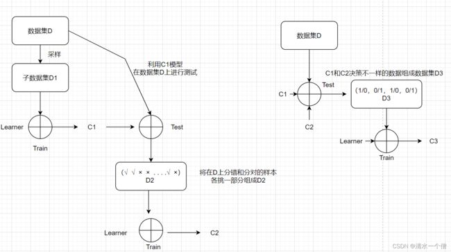
Boosting的决策流程为：

 

AdaBoost算法是Boosting的代表算法，AdaBoost算法指定了权重更新的准则。

Sklearn实现集成学习

下面的代码用Scikit-Learn创建并训练一个投票分类器，由三种不同的分类器组成

from sklearn.model_selection import train_test_split
from sklearn.datasets import make_moons
 
X, y = make_moons(n_samples=500, noise=0.30, random_state=42)
X_train, X_test, y_train, y_test = train_test_split(X, y, random_state=42)
 
 
from sklearn.ensemble import RandomForestClassifier
from sklearn.ensemble import VotingClassifier
from sklearn.linear_model import LogisticRegression
from sklearn.svm import SVC
 
log_clf = LogisticRegression(solver="liblinear", random_state=42)
rnd_clf = RandomForestClassifier(n_estimators=10, random_state=42)
svm_clf = SVC(gamma="auto", random_state=42)
 
voting_clf = VotingClassifier(
    estimators=[('lr', log_clf), ("rf", rnd_clf), ("svc", svm_clf)],
    voting="hard"
)
 
voting_clf.fit(X_train, y_train)
 
from sklearn.metrics import accuracy_score
 
for clf in (log_clf, rnd_clf, svm_clf, voting_clf):
    clf.fit(X_train, y_train)
    y_pred = clf.predict(X_test)
    print(clf.__class__.__name__, accuracy_score(y_test, y_pred))

训练了一个包含500个决策树分类器的集成，每次随机从训练集中采样100个训练实例进行训练，然后放回。

from sklearn.ensemble import BaggingClassifier
from sklearn.tree import DecisionTreeClassifier
 
bag_clf = BaggingClassifier(
    DecisionTreeClassifier(random_state=42), n_estimators=500,
    max_samples=100, bootstrap=True, n_jobs=-1, random_state=42)
bag_clf.fit(X_train, y_train)
y_pred = bag_clf.predict(X_test)
 
 
from sklearn.metrics import accuracy_score
print(accuracy_score(y_test, y_pred))

单个决策树：

tree_clf = DecisionTreeClassifier(random_state=42)
tree_clf.fit(X_train, y_train)
y_pred_tree = tree_clf.predict(X_test)
print(accuracy_score(y_test, y_pred_tree))

结果比较：

from matplotlib.colors import ListedColormap
 
def plot_decision_boundary(clf, X, y, axes=[-1.5, 2.5, -1, 1.5], alpha=0.5, contour=True):
    x1s = np.linspace(axes[0], axes[1], 100)
    x2s = np.linspace(axes[2], axes[3], 100)
    x1, x2 = np.meshgrid(x1s, x2s)
    X_new = np.c_[x1.ravel(), x2.ravel()]
    y_pred = clf.predict(X_new).reshape(x1.shape)
    custom_cmap = ListedColormap(['#fafab0','#9898ff','#a0faa0'])
    plt.contourf(x1, x2, y_pred, alpha=0.3, cmap=custom_cmap)
    if contour:
        custom_cmap2 = ListedColormap(['#7d7d58','#4c4c7f','#507d50'])
        plt.contour(x1, x2, y_pred, cmap=custom_cmap2, alpha=0.8)
    plt.plot(X[:, 0][y==0], X[:, 1][y==0], "yo", alpha=alpha)
    plt.plot(X[:, 0][y==1], X[:, 1][y==1], "bs", alpha=alpha)
    plt.axis(axes)
    plt.xlabel(r"$x_1$", fontsize=18)
    plt.ylabel(r"$x_2$", fontsize=18, rotation=0)
 
plt.figure(figsize=(11,4))
plt.subplot(121)
plot_decision_boundary(tree_clf, X, y)
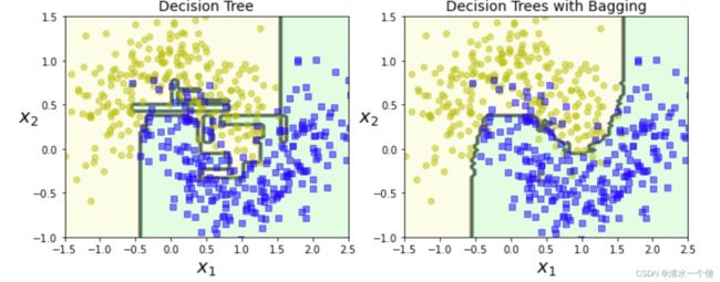
plt.title("Decision Tree", fontsize=14)
plt.subplot(122)
plot_decision_boundary(bag_clf, X, y)
plt.title("Decision Trees with Bagging", fontsize=14)
save_fig("decision_tree_without_and_with_bagging_plot")