实践：基于Softmax回归完成鸢尾花分类任务

        文件内引用的nndl包内的文件代码可翻看以往博客有详细介绍，这么就不详细赘述啦基于Softmax回归的多分类任务_熬夜患者的博客-CSDN博客https://blog.csdn.net/m0_70026215/article/details/133690588?spm=1001.2014.3001.5501

1.数据处理

---

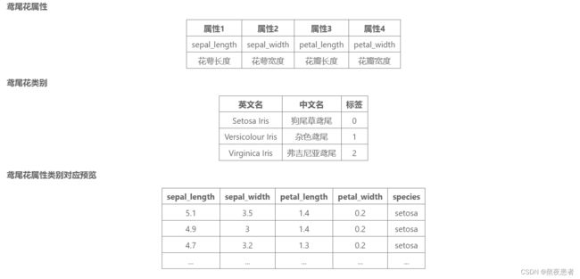
数据集介绍

---

 缺失值分析

from sklearn.datasets import load_iris
import pandas
import numpy as np
import torch


iris_features = np.array(load_iris().data, dtype=np.float32)
iris_labels = np.array(load_iris().target, dtype=np.int32)
print(pandas.isna(iris_features).sum())
print(pandas.isna(iris_labels).sum())

        运行结果:

---

异常值处理

import matplotlib.pyplot as plt #可视化工具

# 箱线图查看异常值分布
def boxplot(features):
    feature_names = ['sepal_length', 'sepal_width', 'petal_length', 'petal_width']

    # 连续画几个图片
    plt.figure(figsize=(5, 5), dpi=200)
    # 子图调整
    plt.subplots_adjust(wspace=0.6)
    # 每个特征画一个箱线图
    for i in range(4):
        plt.subplot(2, 2, i+1)
        # 画箱线图
        plt.boxplot(features[:, i],
                    showmeans=True,
                    whiskerprops={"color":"#E20079", "linewidth":0.4, 'linestyle':"--"},
                    flierprops={"markersize":0.4},
                    meanprops={"markersize":1})
        # 图名
        plt.title(feature_names[i], fontdict={"size":5}, pad=2)
        # y方向刻度
        plt.yticks(fontsize=4, rotation=90)
        plt.tick_params(pad=0.5)
        # x方向刻度
        plt.xticks([])
    plt.savefig('ml-vis.pdf')
    plt.show()

boxplot(iris_features)

         运行结果:

         从输出结果看，数据中基本不存在异常值，所以不需要进行异常值处理。

---

数据读取

def load_data(shuffle=True):
    '''
    加载鸢尾花数据
    输入：
        - shuffle：是否打乱数据，数据类型为bool
    输出：
        - X：特征数据，shape=[150,4]
        - y：标签数据, shape=[150]
    '''
    # 加载原始数据
    X = np.array(load_iris().data, dtype=np.float32)
    y = np.array(load_iris().target, dtype=np.float32)

    X = torch.tensor(X)
    y = torch.tensor(y)

    # 数据归一化
    X_min = torch.min(X, dim=0).values
    X_max = torch.max(X, dim=0).values
    X = (X-X_min) / (X_max-X_min)

    # 如果shuffle为True,随机打乱数据
    if shuffle:
        idx = torch.randperm(X.shape[0])
        X = X[idx]
        y = y[idx]
    return X, y

# 固定随机种子
torch.manual_seed(102)

num_train = 120
num_dev = 15
num_test = 15

X, y = load_data(shuffle=True)
print("X shape: ", X.shape, "y shape: ", y.shape)
X_train, y_train = X[:num_train], y[:num_train]
X_dev, y_dev = X[num_train:num_train + num_dev], y[num_train:num_train + num_dev]
X_test, y_test = X[num_train + num_dev:], y[num_train + num_dev:]

# 打印X_train和y_train的维度
print("X_train shape: ", X_train.shape, "y_train shape: ", y_train.shape)
# 打印前5个数据的标签
print(y_train[:5])

         运行结果:

2.模型构建

from nndl import op

# 输入维度
input_dim = 4
# 类别数
output_dim = 3
# 实例化模型
model = op.model_SR(input_dim=input_dim, output_dim=output_dim)

 3.模型训练

from nndl import op, metric, opitimizer, runner

lr = 0.2

# 梯度下降法
optimizer = opitimizer.SimpleBatchGD(init_lr=lr, model=model)
# 交叉熵损失
loss_fn = op.MultiCrossEntropyLoss()
# 准确率
metric = metric.accuracy

# 实例化RunnerV2
runner = runner.RunnerV2(model, optimizer, metric, loss_fn)

# 启动训练
runner.train([X_train, y_train], [X_dev, y_dev], num_epochs=200, log_epochs=10, save_path="best_model.pdparams")

          运行结果:

        可视化观察训练集与验证集的准确率变化情况。 

from nndl import tools

tools.plot(runner,fig_name='linear-acc3.pdf')

           运行结果:

4.模型评价

runner.load_model('best_model.pdparams')
# 模型评价
score, loss = runner.evaluate([X_test, y_test])
print("[Test] score/loss: {:.4f}/{:.4f}".format(score, loss))

            运行结果: 

 5.模型预测

# 预测测试集数据
logits = runner.predict(X_test)
# 观察其中一条样本的预测结果
pred = torch.argmax(logits[0]).numpy()
print("pred:",pred)
# 获取该样本概率最大的类别
label = y_test[0].numpy()
print("label:",label)
# 输出真实类别与预测类别
print("The true category is {0} and the predicted category is {1}".format(label, pred))

            运行结果: 

 

小结 

到这儿，三、四章的实验就写完了，但是这两天写的有点快，总感觉有些东西没弄的太透彻，但是说不上来是哪部分，总觉得不行，这两天事多，等我这两天忙完的，会把这几个文章全部过一遍，重新翻新一遍，弄透彻！！！！浅浅立个flag！！！加油