读Graph-Matching-Networks复现①嵌入
参数
{'aggregator':
	{'aggregation_type': 'sum',
	 'gated': True,
	 'graph_transform_sizes': [128],
	 'input_size': [32],
	 'node_hidden_sizes': [128]},
 'data':
 	{'dataset_params':
 		{'n_changes_negative': 2,

		 'n_changes_positive': 1,
		 #一对被视为正(相似)的边替换的数量。

		 'n_nodes_range': [20, 20],
		 'p_edge_range': [0.2, 0.2],
		 #生成具有 20 个节点且 p_edge=0.2 (边概率?)的图

		 'validation_dataset_size': 1000},
  	 'problem': 'graph_edit_distance'},
 'encoder':
	 {'edge_hidden_sizes': None,
	  'node_feature_dim': 1,
	  'node_hidden_sizes': [32]},
 'evaluation': {'batch_size': 20},
 'graph_embedding_net':
	 {'edge_hidden_sizes': [64, 64],

	  'edge_net_init_scale': 0.1,
	  #用小参数权重初始化消息 MLP 以防止聚合消息向量爆炸
	  #或者也可以使用例如 层标准化以控制这些的规模。

	  'layer_norm': False,
	  # 在实验中没有使用层范数,但有时会有用

	  'n_prop_layers': 5,
	  'node_hidden_sizes': [64],
	  'node_state_dim': 32,

	  'node_update_type': 'gru',
	  # 其他也可以用'mlp'  `residual`

	  'prop_type': 'matching',
	  #如果用嵌入网络就设置为 `embedding`

	  'reverse_dir_param_different': False,
	  #如果是有向图则设成TRUE

	  'share_prop_params': True,
	  # 判断在信息传递层是否参数共享

	  #如果有双向边就设成FALSE
	  'use_reverse_direction': True},

 'graph_matching_net':
	 {'edge_hidden_sizes': [64, 64],
	  'edge_net_init_scale': 0.1,
	  'layer_norm': False,
	  'n_prop_layers': 5,
	  'node_hidden_sizes': [64],
	  'node_state_dim': 32,
	  'node_update_type': 'gru',
	  'prop_type': 'matching',
	  'reverse_dir_param_different': False,
	  'share_prop_params': True,
	  'similarity': 'dotproduct',
	  'use_reverse_direction': True},
 'model_type': 'embedding',
 'seed': 8,
 'training':
	 {'batch_size': 20,

	  'clip_value': 10.0,
	  #设置梯度裁剪防止梯度爆炸

	  'eval_after': 10,
	  #每个 `eval_after * print_after` 步骤对验证集进行评估。

	  'graph_vec_regularizer_weight': 1e-06,
	  #图向量上有一个小的正则化器会缩放以避免图向量爆炸。
	  #如果模型中的数值问题特别严重,
	  #可以将 `snt.LayerNorm` 添加到每一层的输出、聚合消息和聚合节点表示中,
	  #以将网络激活规模保持在合理范围内。

	  'learning_rate': 0.0001,
	  'loss': 'margin',
	  'margin': 1.0,
	  'mode': 'pair',

	  'n_training_steps': 500000,
	  #控制训练时长

	  'print_after': 100}}
	  #每隔这么多训练步骤打印训练信息
生成固定大小的图
——————
build_datasets划分数据集
(好像训练集或验证集都只有一个图?)
——————————
默认训练模式为’pair’,也即学习结果与标签作误差的标准损失函数(相对于三元损失)
training_data_iter = training_set.pairs(config['training']['batch_size'])
# 'batch_size'为20
first_batch_graphs, _ = next(training_data_iter)
其中
def pairs(self, batch_size):
    """Yields batches of pair data."""
    while True:
        batch_graphs = []
        batch_labels = []
        positive = True
        for _ in range(batch_size):# 20
            g1, g2 = self._get_pair(positive)
            #随意造出的图,依照原图改出的图
            batch_graphs.append((g1, g2))
            #这样的到一批20对图作为一个批次
            batch_labels.append(1 if positive else -1)
            #positive=true对应相似的情况
            positive = not positive
        packed_graphs = self._pack_batch(batch_graphs)
        #_pack_batch将一批图打包成一个collection实例
        labels = np.array(batch_labels, dtype=np.int32)
        yield packed_graphs, labels
        #yield把函数变成一个iter迭代器
其中
def _get_pair(self, positive):
    g = self._get_graph()
    #随机生成一个连通图
    if self._permute:	#True
    #随意定下20个点,再随意添加一些边生成新图
        permuted_g = permute_graph_nodes(g)
    else:
        permuted_g = g
    n_changes = self._k_pos if positive else self._k_neg
    #True → n_changes = 1
    changed_g = substitute_random_edges(g, n_changes)
    #随机删除20条边,再添加n_changes=1条边得到新图
    return permuted_g, changed_g
其中(但是这样100个图里就能返回一个连通图?)
def _get_graph(self):
    """Generate one graph."""
    n_nodes = np.random.randint(self._n_min, self._n_max + 1)
    #其实还是20
    p_edge = np.random.uniform(self._p_min, self._p_max)
    #其实还是0.2

    # 随机生成100个有20个节点以0.2为概率连接的图,再筛选出其中的连通图返回
    n_trials = 100
    for _ in range(n_trials):
        g = nx.erdos_renyi_graph(n_nodes, p_edge)
        if nx.is_connected(g):
            return g
def _pack_batch(self, graphs):
    Graphs = []
    for graph in graphs:
        for inergraph in graph:
            Graphs.append(inergraph)
    graphs = Graphs
    #一批共40个图
    from_idx = []
    to_idx = []
    graph_idx = []
    n_total_nodes = 0
    n_total_edges = 0
    for i, g in enumerate(graphs):
        n_nodes = g.number_of_nodes()
        n_edges = g.number_of_edges()
        edges = np.array(g.edges(), dtype=np.int32)
        #from_idx记录所有边的起点
        from_idx.append(edges[:, 0] + n_total_nodes)
        #to_idx记录所有边的终点
        to_idx.append(edges[:, 1] + n_total_nodes)
        #记录全为当前图索引i的向量(长20)
        graph_idx.append(np.ones(n_nodes, dtype=np.int32) * i)
        n_total_nodes += n_nodes
        n_total_edges += n_edges
    GraphData = collections.namedtuple('GraphData', [
        'from_idx',
        'to_idx',
        'node_features',
        'edge_features',
        'graph_idx',
        'n_graphs'])
    return GraphData(
        from_idx=np.concatenate(from_idx, axis=0),
        to_idx=np.concatenate(to_idx, axis=0),
        # this task only cares about the structures, the graphs have no features.
        # setting higher dimension of ones to confirm code functioning
        # with high dimensional features.
        node_features=np.ones((n_total_nodes, 8), dtype=np.float32),
        edge_features=np.ones((n_total_edges, 4), dtype=np.float32),
        graph_idx=np.concatenate(graph_idx, axis=0),
        n_graphs=len(graphs),
    )
(用yield是节省了空间,但时间上还挺久的)
以training_data_iter的第一个,即next(training_data_iter)为例
packed_graphs,即next(training_data_iter)[0]为
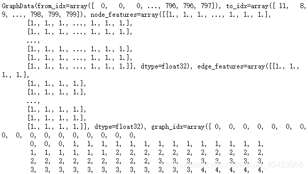
其中from_idx和to_idx为长度相同但不定的行向量,即边的起点索引集和终点索引集,这第一个长为1552,
edge_features是长度与其相同也不定的4维行向量,该不定长度即边总数大概1480~1690,这第一个长为1552,即1552x4
node_features是全1的800长(即节点总数)的8维行向量,即800x8
graph_idx是800长的行向量
n_graphs为40
labels,即next(training_data_iter)[1]为
[ 1 -1 1 -1 1 -1 1 -1 1 -1 1 -1 1 -1 1 -1 1 -1 1 -1],长20
————————————————
将packed_graphs记作first_batch_graphs,(莫名其妙)取两个_features的列数,即8和4分别作为参数node_feature_dim,edge_feature_dim构造模型
这里先用图嵌入,也即是GNN来试试
GraphEmbeddingNet(
  (_encoder): GraphEncoder(
    (MLP1): Sequential(
      (0): Linear(in_features=8, out_features=32, bias=True)
    )
    (MLP2): Sequential(
      (0): Linear(in_features=4, out_features=16, bias=True)
    )
  )
  (_aggregator): GraphAggregator(
    (MLP1): Sequential(
      (0): Linear(in_features=32, out_features=256, bias=True)
    )
    (MLP2): Sequential(
      (0): Linear(in_features=128, out_features=128, bias=True)
    )
  )
  (_prop_layers): ModuleList(
    (0): GraphPropLayer(
      (_message_net): Sequential(
        (0): Linear(in_features=80, out_features=64, bias=True)
        (1): ReLU()
        (2): Linear(in_features=64, out_features=64, bias=True)
      )
      (_reverse_message_net): Sequential(
        (0): Linear(in_features=80, out_features=64, bias=True)
        (1): ReLU()
        (2): Linear(in_features=64, out_features=64, bias=True)
      )
      (GRU): GRU(64, 32)
    )
    (1): GraphPropLayer(
      (_message_net): Sequential(
        (0): Linear(in_features=80, out_features=64, bias=True)
        (1): ReLU()
        (2): Linear(in_features=64, out_features=64, bias=True)
      )
      (_reverse_message_net): Sequential(
        (0): Linear(in_features=80, out_features=64, bias=True)
        (1): ReLU()
        (2): Linear(in_features=64, out_features=64, bias=True)
      )
      (GRU): GRU(64, 32)
    )
    (2): GraphPropLayer(
      (_message_net): Sequential(
        (0): Linear(in_features=80, out_features=64, bias=True)
        (1): ReLU()
        (2): Linear(in_features=64, out_features=64, bias=True)
      )
      (_reverse_message_net): Sequential(
        (0): Linear(in_features=80, out_features=64, bias=True)
        (1): ReLU()
        (2): Linear(in_features=64, out_features=64, bias=True)
      )
      (GRU): GRU(64, 32)
    )
    (3): GraphPropLayer(
      (_message_net): Sequential(
        (0): Linear(in_features=80, out_features=64, bias=True)
        (1): ReLU()
        (2): Linear(in_features=64, out_features=64, bias=True)
      )
      (_reverse_message_net): Sequential(
        (0): Linear(in_features=80, out_features=64, bias=True)
        (1): ReLU()
        (2): Linear(in_features=64, out_features=64, bias=True)
      )
      (GRU): GRU(64, 32)
    )
    (4): GraphPropLayer(
      (_message_net): Sequential(
        (0): Linear(in_features=80, out_features=64, bias=True)
        (1): ReLU()
        (2): Linear(in_features=64, out_features=64, bias=True)
      )
      (_reverse_message_net): Sequential(
        (0): Linear(in_features=80, out_features=64, bias=True)
        (1): ReLU()
        (2): Linear(in_features=64, out_features=64, bias=True)
      )
      (GRU): GRU(64, 32)
    )
  )
)
#创建可以给无key字典提供默认值的字典
accumulated_metrics = collections.defaultdict(list)
#此时结果为defaultdict(list, {})
成对比较,所以记training_n_graphs_in_batch *= 2=40
迭代开始:
1.提取出来node_features, edge_features, from_idx, to_idx, graph_idx, labels,先tensor化,再cuda化
2.送进model前向(GraphEmbeddingNet)
①先送进GraphEncoder前向,也即将两个_features分别通过两个MLP,输出node_features, edge_features尺寸由分别的hidden_sizes决定,
node_states = node_features
layer_outputs = [node_states]
②五层prop层(考虑信息的双向传递,每个方向是一层MLP接ReLu激活后再接一个MLP)
每层更新node_states,记录进layer_outputs
至于边信息,在GraphPropLayer的前向过程中_compute_aggregated_messages》graph_prop_once中edge_features与from_states和to_states拼接得到的edge_inputs整合出messages传入unsorted_segment_sum得到正向的aggregated_messages,同理得到反向的reverse_aggregated_messages与前者相加得到aggregated_messages,进而送入_compute_node_update与节点信息整合
从而GraphPropLayer在GraphEmbeddingNet》_build_layer》_build_layer中构造prop层的结构
③最后通过aggregator层整合节点信息
首先是一层MLP得到800x256的矩阵node_states_g,
if self._gated:	#True
     gates = torch.sigmoid(node_states_g[:, :self._graph_state_dim])
     #	前128列通过sigmoid的800x128的结果乘以后128列
     node_states_g = node_states_g[:, self._graph_state_dim:] * gates
接着计算张量段的和
graph_states = unsorted_segment_sum(node_states_g, graph_idx, n_graphs)
其中判定len(graph_idx.shape)=1,则
s=torch.prod(torch.tensor(node_states_g.shape[1:])).long().cuda(),即tensor(128,device=‘cuda:0’),把graph_idx横向复制成800x128的矩阵segment_idstensor = torch.zeros(*shape).cuda().scatter_add(0, segment_ids,node_states_g)这里scatter_add参考https://blog.csdn.net/weixin_43922901/article/details/102587924的二维计算
torch.zeros(*shape).cuda()[segment_ids[i][j]][j] +=
node_states_g[i][j] # 0维上的运算
torch.zeros(*shape).cuda()[i][segment_ids[i][j]] +=
node_states_g[i][j] # 1维上
最终统一tensor为node_states_g的数据类型,返回tensor,即graph_states
(由于_aggregation_type设为sum所以跳过将小于 -1e5 的所有内容重置为 0进一步转换减少的graph_states这一过程)
将graph_states送进第二个MLP,最终得到整个模型的输出graph_vectors 40x128
接下来把graph_vectors横向劈开得到上下两个20x128,记作x和y
进而计算成对损失,可以是margin距离,即 t o r c h . r e l u [ m a r g i n − l a b e l s ∗ ( 1 − ∣ ∣ x , y ∣ ∣ 2 ) ] torch.relu[margin - labels * (1 -||x, y||_2)] torch.relu[margin−labels∗(1−∣∣x,y∣∣2)],margin可以取1
或者hamming距离,首先如下计算x和y的近似汉明相似度(不太懂两个tanh的内积能等效于异或xor吗,还求个均值是怎样)
def approximate_hamming_similarity(x, y):
    """Approximate Hamming similarity."""
    return torch.mean(torch.tanh(x) * torch.tanh(y), dim=1)
然后计算距离 0.25 × [ l a b e l s − a p p r o x i m a t e _ h a m m i n g _ s i m i l a r i t y ( x , y ) ] 2 0.25×[labels - approximate\_hamming\_similarity(x, y)]^2 0.25×[labels−approximate_hamming_similarity(x,y)]2
接着记录相似样本和非相似样本的位置is_pos,is_neg
之后是相似度,可以是margin相似度,即负的相似度;也可以是如下汉明相似度(这次整个x y中正数相乘也是不懂)
def exact_hamming_similarity(x, y):
    """Compute the binary Hamming similarity."""
    match = ((x > 0) * (y > 0)).float()
    return torch.mean(match, dim=1)
(下面两步也不明白是在干啥)
sim_pos = torch.sum(sim * is_pos) / (n_pos + 1e-8)
sim_neg = torch.sum(sim * is_neg) / (n_neg + 1e-8)
然后(依然不懂)
graph_vec_scale = torch.mean(graph_vectors ** 2)
loss += (config['training']['graph_vec_regularizer_weight'] *0.5 * graph_vec_scale)
# config['training']['graph_vec_regularizer_weight']=1e-6
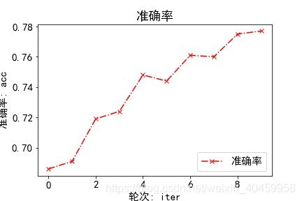
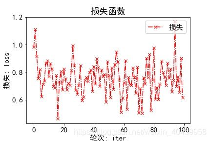
接着就是BP优化的事了,顺便记录进accumulated_metrics,方便后续打印(不过这时loss还是矩阵的形式,这给后续画图的打算添了不少麻烦,按说记录损失值才对吧,记成一个矩阵耗复杂度不说,关键这样对吗?)
(试着画了下图感觉BP时使用loss均值还是原loss的影响不大,ACC和AUC是挺漂亮的,总体上升明显,但loss波动的仿佛没有收敛)
至于评估阶段eval,每1000轮一次,
首先是计算AUC即ROC曲线面积,
这里with torch.no_grad():是让这一块的代码不做计算图(就是链式法则),体现在这一段的变量没有grad_fn=
通过一次model前向得到x和y,直接compute_similarity计算相似度scores
scores = (scores - scores_min) / (scores_max - scores_min + 1e-8)
labels = (labels + 1) / 2
如上整理后送入sklearn的metrics.roc_curve算出auc值
(ACC后面看到三元损失训练时再细扣这里吧)

————————————
或者采用三元损失,
training_data_iter = training_set.triplets(config['training']['batch_size'])
first_batch_graphs = next(training_data_iter)
其中
def triplets(self, batch_size):
    """Yields batches of triplet data."""
    while True:
        batch_graphs = []
        for _ in range(batch_size):
            g1, g2, g3 = self._get_triplet()
            batch_graphs.append((g1, g2, g1, g3))
        yield self._pack_batch(batch_graphs)
与pairs的区别在于没有标签,以及存进batch的顺序
其中
def _get_triplet(self):
   """Generate one triplet of graphs."""
   g = self._get_graph()
   if self._permute:
       permuted_g = permute_graph_nodes(g)
   else:
       permuted_g = g
   pos_g = substitute_random_edges(g, self._k_pos) #1
   neg_g = substitute_random_edges(g, self._k_neg) #2
   return permuted_g, pos_g, neg_g
与_get_pair的区别体现在用substitute_random_edges构造了两个图,一个天了一条边,另一个添了两条

from_idx,to_idx 3360
edge_features 3360x4
node_features 1600x8
从而送进model得到80x128的graph_vectors
通过reshape_and_split_tensor切分出4份x_1, y, x_2, z计算损失(其实x_1=x_2)
margin: t o r c h . r e l u ( m a r g i n + ∣ ∣ x 1 − y ∣ ∣ 2 − ∣ ∣ x 2 − z ∣ ∣ 2 torch.relu(margin+||x_1-y||_2 -||x_2-z||_2 torch.relu(margin+∣∣x1−y∣∣2−∣∣x2−z∣∣2
hamming: 0.125 × { [ a p p r o x i m a t e _ h a m m i n g _ s i m i l a r i t y ( x 1 , y ) − 1 ] 2 + [ a p p r o x i m a t e _ h a m m i n g _ s i m i l a r i t y ( x 2 , z ) + 1 ] 2 } 0.125×\{[approximate\_hamming\_similarity(x_1, y) - 1] ^2 +[approximate\_hamming\_similarity(x_2, z) + 1]^2\} 0.125×{[approximate_hamming_similarity(x1,y)−1]2+[approximate_hamming_similarity(x2,z)+1]2}
sim_pos = torch.mean(compute_similarity(config, x_1, y))
sim_neg = torch.mean(compute_similarity(config, x_2, z))
graph_vec_scale = torch.mean(graph_vectors ** 2)
loss += (config['training']['graph_vec_regularizer_weight'] *0.5 * graph_vec_scale)
接着评估阶段计算准确率,大概因为成对损失本身就能表征准确率,所以统一采用三元损失的方式来计算准确率,
这时通过前向得到x_1, y, x_2, z,再分别计算应该相似的x_1和y以及应该不相似的x_2和z的相似度sim_1和sim_2
得到sim_1 > sim_2的01向量,求均值作为acc
————————————
优化器
Adam (
Parameter Group 0
    amsgrad: False
    betas: (0.9, 0.999)
    eps: 1e-08
    lr: 0.0001
    weight_decay: 1e-05
)
os.environ["CUDA_DEVICE_ORDER"] = "PCI_BUS_ID"
os.environ["CUDA_VISIBLE_DEVICES"] = "0"
use_cuda = torch.cuda.is_available()
device = torch.device('cuda' if use_cuda else 'cpu')
model.to(device)