cp16_Model Sequential_Output_Hidden_Recurrent NNs_LSTM_aclImdb_IMDb_Embed_token_py_function_GRU_Gate

     In the previous chapter cp15_Classifying Images with Deep Convolutional NN_Loss_Cross Entropy_ax.text_mnist_ CelebA_Colab_ck https://blog.csdn.net/Linli522362242/article/details/108414534, we focused on convolutional neural networks (CNNs). We covered the building blocks of CNN architectures and how to implement deep CNNs in TensorFlow. Finally, you learned how to use CNNs for image classification. In this chapter, we will explore recurrent neural networks 递归神经网络, 循环神经网络(RNNs) and see their application in modeling sequential data.

We will cover the following topics:

• • Introducing sequential data
• • RNNs for modeling sequences
• • Long short-term memory (LSTM)
• • Truncated backpropagation through time (TBPTT)
• • Implementing a multilayer RNN for sequence modeling in TensorFlow
• • Project one: RNN sentiment analysis of the IMDb movie review dataset
• • Project two: RNN character-level language modeling with LSTM cells, using text data from Jules Verne's The Mysterious Island
• • Using gradient clipping to avoid exploding gradients
• • Introducing the Transformer model and understanding the self-attention mechanism

Introducing sequential data

     Let's begin our discussion of RNNs by looking at the nature of sequential data, which is more commonly known as sequence data or sequences. We will take a look at the unique properties of sequences that make them different to other kinds of data. We will then see how we can represent sequential data and explore the various categories of models for sequential data, which are based on the input and output of a model. This will help us to explore the relationship between RNNs and sequences in this chapter.

Modeling sequential data – order matters

     What makes sequences unique, compared to other types of data, is that elements in a sequence appear in a certain order and are not independent of each other.
Typical machine learning algorithms for supervised learning assume that the input is independent and identically distributed (IID) data, which means that the training examples are mutually independent and have the same underlying distribution. In this regard, based on the mutual independence assumption, the order in which the training examples are given to the model is irrelevant. For example, if we have a sample consisting of n training examples, , the order in which we use the data for training our machine learning algorithm does not matter. An example of this scenario would be the Iris dataset that we previously worked with. In the Iris dataset, each flower has been measured independently, and the measurements of one flower do not influence the measurements of another flower.

     However, this assumption is not valid when we deal with sequences—by definition, order matters. Predicting the market value of a particular stock would
be an example of this scenario. For instance, assume we have a sample of n training examples, where each training example represents the market value of a certain
stock on a particular day. If our task is to predict the stock market value for the next three days, it would make sense to consider the previous stock prices in a date-sorted order to derive trends rather than utilize these training examples in a randomized order.
###############################################
Sequential data versus time-series data

     Time-series data is a special type of sequential data, where each example is associated with a dimension for time. In time-series data, samples are taken at successive[səkˈsesɪv]连续的 time stamps, and therefore, the time dimension determines the order among the data points. For example, stock prices and voice or speech records are timeseries data.

     On the other hand, not all sequential data has the time dimension, for example, text data or DNA sequences, where the examples are ordered but they do not qualify as time-series data. As you will see, in this chapter, we will cover some examples of natural language processing (NLP) and text modeling that are not time-series data, but note that RNNs can also be used for time-series data.
###############################################

Representing sequences

     We've established that order among data points is important in sequential data, so we next need to find a way to leverage this ordering information in a machine learning model. Throughout this chapter, we will represent sequences as 〈〉 . The superscript indices indicate the order of the instances, and the length of the sequence is T. For a sensible example of sequences, consider time-series data, where each example point, , belongs to a particular time, t. The following figure shows an example of time-series data where both the input features (x's) and the target labels (y's) naturally follow the order according to their time axis; therefore, both the x's and y's are sequences:

     As we have already mentioned, the standard neural network (NN) models that we have covered so far, such as multilayer perceptron (MLP) and CNNs for image data, assume that the training examples are independent of each other and thus do not incorporate ordering information. We can say that such models do not have a memory of previously seen training examples. For instance, the samples are passed through the feedforward and backpropagation steps, and the weights are updated independently of the order in which the training examples are processed.

     RNNs(recurrent neural networks), by contrast, are designed for modeling sequences and are capable of remembering past information and processing new events accordingly, which is a clear advantage when working with sequence data.

The different categories of sequence modeling

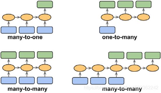
     Sequence modeling has many fascinating applications, such as language translation (for example, translating text from English to German), image captioning, and text generation. However, in order to choose an appropriate architecture and approach, we have to understand and be able to distinguish between these different sequence modeling tasks. The following figure, based on the explanations in the excellent article The Unreasonable Effectiveness of Recurrent Neural Networks, by Andrej Karpathy (http://karpathy.github.io/2015/05/21/rnn-effectiveness/), summarizes the most common sequence modeling tasks, which depend on the relationship categories of input and output data:

VS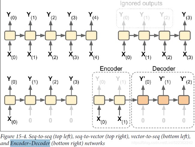 
     Let's discuss the different relationship categories between input and output data, which were depicted in the previous figure, in more detail. If neither the input nor
output data represents sequences, then we are dealing with standard data, and we could simply use a multilayer perceptron (or another classification model previously
covered in this book) to model such data. However, if either the input or output is a sequence, the modeling task likely falls into one of these categories:

• • Many-to-one: The input data is a sequence, but the output is a fixed-size vector or scalar, not a sequence. For example, in sentiment analysis, the input is text-based (for example, a movie review) and the output is a class label (for example, a label denoting whether a reviewer liked the movie).
  https://towardsdatascience.com/illustrated-guide-to-recurrent-neural-networks-79e5eb8049c9
• • One-to-many: The input data is in standard format and not a sequence, but the output is a sequence. An example of this category is image captioning—the input is an image and the output is an English phrase summarizing the content of that image.
   
• • Many-to-many: Both the input and output arrays are sequences. This category can be further divided based on whether the input and output are synchronize['sɪŋkrənaɪzd]同步的. An example of a synchronized many-to-many modeling task is video classification, where each frame in a video is labeled. An example of a delayed many-to-many modeling task would be translating one language into another. For instance, an entire English sentence must be read and processed by a machine before its translation into German is produced.

Now, after summarizing the three broad categories of sequence modeling, we can move forward to discussing the structure of an RNN.

RNNs for modeling sequences

     In this section, before we start implementing RNNs in TensorFlow, we will discuss the main concepts of RNNs. We will begin by looking at the typical structure of an RNN, which includes a recursive component to model sequence data. Then, we will examine how the neuron activations are computed in a typical RNN. This will create a context for us to discuss the common challenges in training RNNs, and we will then discuss solutions to these challenges, such as LSTM(Long short-term memory) and gated recurrent units (GRUs).

Understanding the RNN looping mechanism

     Let's start with the architecture of an RNN. The following figure shows a standard feedforward NN and an RNN side by side for comparison:

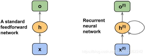
     Both of these networks have only one hidden layer. In this representation, the units are not displayed, but we assume that the input layer (x), hidden layer (h), and
output layer (o) are vectors that contain many units.
#########################################

Determining the type of output from an RNN

     This generic RNN architecture could correspond to the two sequence modeling categories where the input is a sequence. Typically, a recurrent layer can return a sequence as output,〈〉 , or simply return the last output (at t = T, that is, ). Thus, it could be either many-to-many, or it could be many-to-one if, for example, we only use the last element, , as the final output.

     As you will see later, in the TensorFlow Keras API, the behavior of a recurrent layer with respect to returning a sequence as output or simply using the last output can be specified by setting the argument return_sequences to True or False, respectively.
#########################################

     In a standard feedforward network, information flows from the input to the hidden layer, and then from the hidden layer to the output layer. On the other hand, in an RNN, the hidden layer receives its input from both the input layer of the current time step and the hidden layer from the previous time step.

     The flow of information in adjacent time steps in the hidden layer allows the network to have a memory of past events. This flow of information is usually displayed as a loop, also known as a recurrent edge in graph notation, which is how this general RNN architecture got its name.

     Similar to multilayer perceptrons, RNNs can consist of multiple hidden layers. Note that it's a common convention to refer to RNNs with one hidden layer as a singlelayer RNN, which is not to be confused with single-layer NNs without a hidden layer, such as Adaline or logistic regression. The following figure illustrates an RNN with one hidden layer (top) and an RNN with two hidden layers (bottom):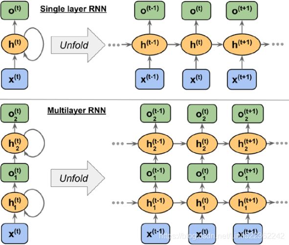

     In order to examine the architecture of RNNs and the flow of information, a compact representation with a recurrent edge can be unfolded, which you can see in the
preceding figure.

     As we know, each hidden unit in a standard NN receives only one input—the net preactivation(or net inputs(z) in activation function ) associated with the input layer. In contrast, each hidden unit in an RNN receives two distinct sets of input—the preactivation from the input layer and the activation of the same hidden layer from the previous time step, t – 1.

     At the first time step, t = 0, the hidden units are initialized to zeros or small random values. Then, at a time step where t > 0, the hidden units receive their input from the data point at the current time t,  (contains several feature columns), and the previous values of hidden units at t – 1, indicated as .

Similarly, in the case of a multilayer RNN, we can summarize the information flow as follows:

• layer = 1: Here, the hidden layer is represented as and it receives its input from the data point, , and the hidden values in the same layer, but at the

previous time step, .

• layer = 2: The second hidden layer, , receives its inputs from the outputs of the layer below at the current time step () and its own hidden values

from the previous time step, .

     Since, in this case, each recurrent layer must receive a sequence as input, all the recurrent layers except the last one must return a sequence as output (that is,
return_sequences=True). The behavior of the last recurrent layer depends on the type of problem.

Computing activations in an RNN

     Now that you understand the structure and general flow of information in an RNN, let's get more specific and compute the actual activations of the hidden layers, as well as the output layer. For simplicity, we will consider just a single hidden layer; however, the same concept applies to multilayer RNNs.

     Each directed edge (the connections between boxes) in the representation of an RNN that we just looked at is associated with a weight matrix. Those weights do not depend on time, t; therefore, they are shared across the time axis. The different weight matrices in a single-layer RNN are as follows:

• • : The weight matrix between the input, , and the hidden layer, h
• • : The weight matrix associated with the recurrent edge
• • : The weight matrix between the hidden layer and output layer

These weight matrices are depicted in the following figure: (hidden-to-hidden recurrence)
a weight matrix is shared across the time axis.
     In certain implementations, you may observe that the weight matrices, and , are concatenated to a combined matrix, = [; ] . Later in this section, we will make use of this notation as well.

     Computing the activations is very similar to standard multilayer perceptrons and other types of feedforward NNs. For the hidden layer, the net input, (preactivation), is computed through a linear combination, that is, we compute the sum of the multiplications of the weight matrices with the corresponding vectors and add the bias unit:

Then, the activations of the hidden units at the time step, t, are calculated as follows:

Here, is the bias vector for the hidden units and is the activation function of the hidden layer.

In case you want to use the concatenated weight matrix, = [; ] , the formula for computing hidden units will change, as follows:

     Once the activations of the hidden units at the current time step are computed, then the activations of the output units will be computed, as follows:

To help clarify this further, the following figure shows the process of computing these activations with both formulations:
hidden-to-hidden recurrence ###############################################
Training RNNs using backpropogation through time (BPTT)

     The learning algorithm for RNNs was introduced in 1990: Backpropagation Through Time: What It Does and How to Do It (Paul Werbos, Proceedings of IEEE, 78(10): 1550-1560, 1990).

     To train an RNN, the trick is to unroll it through time (like we just did) and then simply use regular backpropagation (see Figure 15-5). This strategy is called backpropagation through time (BPTT).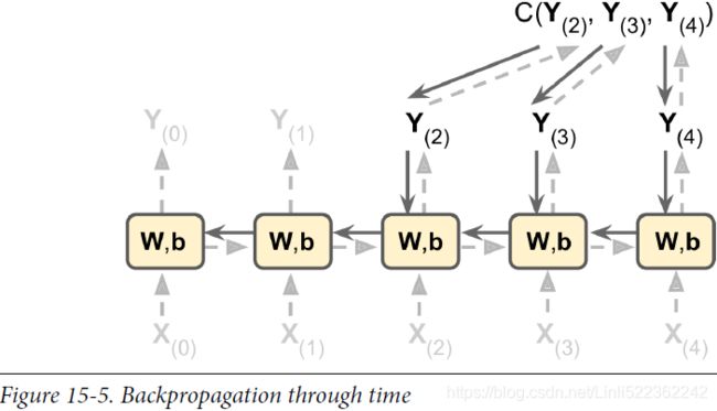

     Just like in regular backpropagation, there is a first forward pass through the unrolled network (represented by the dashed arrows). Then the output sequence is evaluated using a cost function (where T is the max time step). Note that this cost function may ignore some outputs, as shown in Figure 15-5 (for example, in a sequence-to-vector RNN, all outputs are ignored except for the very last one). The gradients of that cost function are then propagated backward through the unrolled network (represented by the solid arrows). Finally the model parameters are updated using the gradients computed during BPTT. Note that the gradients flow backward through all the outputs used by the cost function, not just through the final output (for example, in Figure 15-5 the cost function is computed using the last three outputs of the network, Y(2), Y(3), and Y(4), so gradients flow through these three outputs, but not through Y(0) and Y(1)). Moreover, since the same parameters W and b are used at each time step, backpropagation will do the right thing and sum over all time steps.

     The derivation of the gradients might be a bit complicated, but the basic idea is that the overall loss, L, is the sum of all the loss functions at times t = 1 to t = T:
 OR https://arxiv.org/pdf/1211.5063.pdf
https://arxiv.org/pdf/1211.5063.pdf
     Since the loss at time t is dependent on the hidden units at all previous time steps 1 : t,
the gradient will be computed as follows:
Here,  is computed as a multiplication of adjacent time steps: 
https://arxiv.org/pdf/1211.5063.pdf
###############################################

Hidden-recurrence versus output-recurrence

     So far, you have seen recurrent networks in which the hidden layer has the recurrent property. However, note that there is an alternative model in which the recurrent
connection comes from the output layer. In this case, the net activations from the output layer at the previous time step, , can be added in one of two ways:

• • To the hidden layer at the current time step, (shown in the following figure as output-to-hidden recurrence)
• • To the output layer at the current time step, (shown in the following figure as output-to-output recurrence)
  

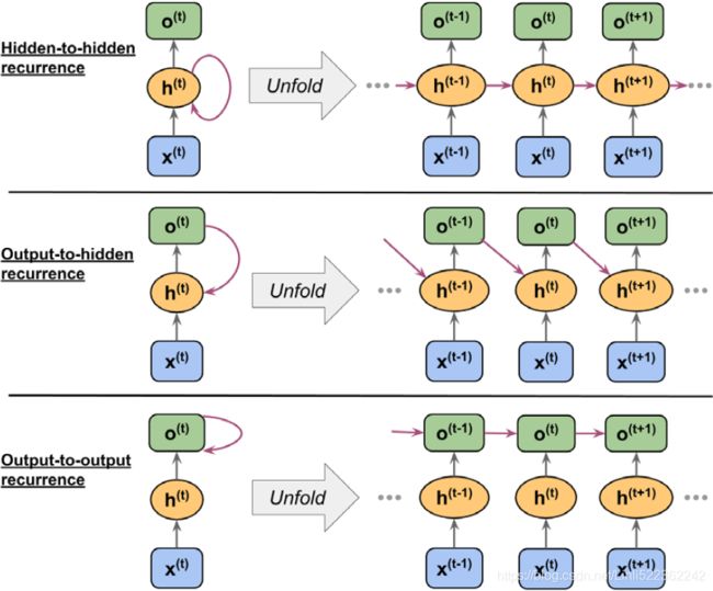
     As shown in the previous figure, the differences between these architectures can be clearly seen in the recurring connections. Following our notation, the weights associated with the recurrent connection will be denoted for the hidden-to-hidden recurrence by , for the output-to-hidden recurrence by , and for the output-to-output recurrence by . In some articles in literature, the weights associated with the recurrent connections are also denoted by .

     To see how this works in practice, let's manually compute the forward pass for one of these recurrent types. Using the TensorFlow Keras API, a recurrent layer can be defined via SimpleRNN, which is similar to the output-to-output recurrence. In the following code, we will create a recurrent layer from SimpleRNN and perform a forward pass on an input sequence of length 3 to compute the output. We will also manually compute the forward pass and compare the results with those of SimpleRNN. First, let's create the layer and assign the weights for our manual computations:
################################################

tf.keras.layers.SimpleRNN(
    units, activation='tanh', use_bias=True,
    kernel_initializer='glorot_uniform',
    recurrent_initializer='orthogonal',
    bias_initializer='zeros', kernel_regularizer=None,
    recurrent_regularizer=None, bias_regularizer=None, activity_regularizer=None,
    kernel_constraint=None, recurrent_constraint=None, bias_constraint=None,
    dropout=0.0, recurrent_dropout=0.0, return_sequences=False, return_state=False,
    go_backwards=False, stateful=False, unroll=False, **kwargs
)

units : Positive integer, dimensionality of the output space.
################################################

output-to-output recurrence

import tensorflow as tf
tf.random.set_seed(1)

rnn_layer = tf.keras.layers.SimpleRNN( # output-to-output recurrence
    units=2, use_bias=True,
    return_sequences=True
)
# The input shape for this layer is (None, None, 5), where 
# the first dimension is the batch dimension (using None for variable batch size), 
# the second dimension corresponds to the sequence (using None for the variable sequence length),
# and the last dimension corresponds to the features.
rnn_layer.build( input_shape=(None,None,5) )

w_xh, w_oo, b_h = rnn_layer.weights

print('W_xh shape:', w_xh.shape)
print('W_oo shape:', w_oo.shape) #the weight is associated with the output-to-output recurrence
print('b_h shape:', b_h.shape)

According to the formula, the weights( W_xh, W_hh and W_oo) and bias vector must be transposed 

     The input shape for this layer is (None, None, 5), where

• the first dimension is the batch dimension (using None for variable batch size),
   
• the second dimension corresponds to the sequence (using None for the variable sequence length), and
   
• the last dimension corresponds to the features. Notice that we set return_sequences=True, which, for an input sequence of length 3, will result in the output sequence . Otherwise, it would only return the final output, .

Now, we will call the forward pass on the rnn_layer and manually compute the outputs at each time step and compare them:

x_seq = tf.convert_to_tensor(
    [[1.0]*5, # 5 is the number of features
     [2.0]*5, # the number of rows is the variable sequence length
     [3.0]*5
    ],
    dtype=tf.float32
)
x_seq

 

### output of SimpleRNN:
# tf.reshape( x_seq, shape=(1,3,5) )
# 
output = rnn_layer( tf.reshape( x_seq, shape=(1,3,5) ) )
output

output.shape

 : 1 batches, 3 sequences, 2 units(dimensionality of the output space)

# manually computing the output

# manually computing the output:
out_to_out = []
for t in range( len(x_seq) ):
    xt = tf.reshape( x_seq[t], (1,5) )
    print( "Time step {} =>".format(t) )
    print( '   Input           :', xt.numpy() )
    
    ht = tf.matmul(xt, w_xh) + b_h         ###########
    print('   Hidden          :', ht.numpy())
    
    if t>0:
        prev_output = out_to_out[t-1]
    else:
        prev_output = tf.zeros(shape=(ht.shape))
    
    ot = ht + tf.matmul(prev_output, w_oo) ###########
    ot = tf.math.tanh(ot) # since the activation in SimpleRNN is 'tanh'
    out_to_out.append(ot)
    
    print('   Output (manual) :', ot.numpy())
    print('   SimpleRNN output: '.format(t), 
          output[0][t].numpy())
    print()

  <== 
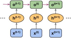
 VS
     In our manual forward computation, we used the hyperbolic tangent (tanh) activation function, since it is also used in SimpleRNN (the default activation). As you can see from the printed results, the outputs from the manual forward computations exactly match the output of the SimpleRNN layer at each time step. Hopefully, this hands-on task has enlightened you on the mysteries of recurrent networks.

The challenges of learning long-range interactions

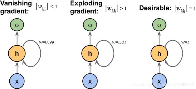
    BPTT (backpropogation through time), which was briefly mentioned earlier, introduces some new challenges. Because of the multiplicative factor, , in computing the gradients of a loss function, the so-called vanishing and exploding gradient problems arise. These problems are explained by the examples in the following figure, which shows an RNN with only one hidden unit for simplicity:
vs  <=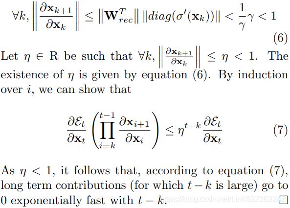
     Basically, has t – k multiplications; therefore, multiplying the w (OR ), by itself t – k times results in a factor,  (OR ). As a result, if || < 1 , this factor (OR )becomes very small (layers that get a small gradient update stops learning. ) when t – k is large. On the other hand, if the weight of the recurrent edge is || > 1 , then becomes very large when t – k is large. Note that large t – k refers to long-range dependencies. We can see that a naive solution to avoid vanishing or exploding gradients can be reached by ensuring || = 1 . If you are interested and would like to investigate this in more detail, read On the difficulty of training recurrent neural networks, by R. Pascanu, T. Mikolov, and Y. Bengio, 2012 (https://arxiv.org/pdf/1211.5063.pdf ：On the difficulty of training Recurrent Neural Networks).

In practice, there are at least three solutions to this problem:
• Gradient clipping
• TBPTT(Truncated backpropagation through time)
• LSTM(Long short-term memory cells)

     Using gradient clipping, we specify a cut-off or threshold value for the gradients, and we assign this cut-off value to gradient values that exceed this value. In contrast, TBPTT simply limits the number of time steps that the signal can backpropagate after each forward pass. For example, even if the sequence has 100 elements or steps, we may only backpropagate the most recent 20 time steps.

     While both gradient clipping and TBPTT can solve the exploding gradient problem, the truncation limits the number of steps that the gradient can effectively flow back
and properly update the weights. On the other hand, LSTM, designed in 1997 by Sepp Hochreiter and Jürgen Schmidhuber, has been more successful in vanishing
and exploding gradient problems while modeling long-range dependencies through the use of memory cells. Let's discuss LSTM in more detail.

Long short-term memory cells

     As stated previously, LSTMs were first introduced to overcome the vanishing gradient problem (Long Short-Term Memory, S. Hochreiter and J. Schmidhuber, Neural
Computation, 9(8): 1735-1780, 1997). The building block of an LSTM is a memory cell, which essentially represents or replaces the hidden layer of standard RNNs.

     In each memory cell, there is a recurrent edge that has the desirable weight, w = 1, as we discussed, to overcome the vanishing and exploding gradient problems. The
values associated with this recurrent edge are collectively called the cell state. The unfolded structure of a modern LSTM cell is shown in the following figure: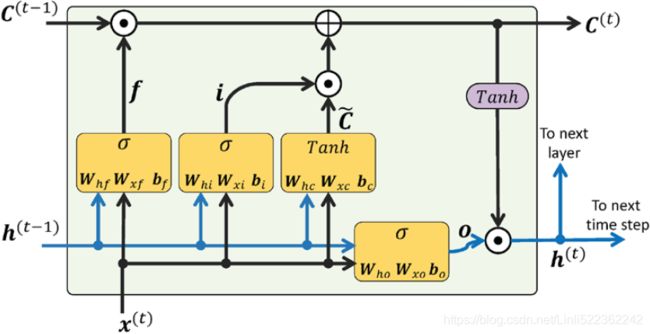
OR
Notice that the cell state from the previous time step, , is modified to get the cell state at the current time step, , without being multiplied directly with any weight factor. The flow of information in this memory cell is controlled by several computation units (often called gates) that will be described here. In the previous figure, ⊙ refers to the element-wise product (element-wise multiplication) and ⨁ means element-wise summation (element-wise addition). Furthermore, refers to the input data at time t, and indicates the hidden units at time t – 1. Four boxes are indicated with an activation function, either the sigmoid function ###( it squishes values between 0 and 1, That is helpful to update or forget data because any number getting multiplied by 0 is 0, causing values to disappears or be “forgotten.” Any number multiplied by 1 is the same value therefore that value stay’s the same or is “kept.” The network can learn which data is not important therefore can be forgotten or which data is important to keep. ) or tanh(The tanh function squishes values to always be between -1 and 1.), ###and a set of weights; these boxes apply a linear combination by performing matrix-vector multiplications on their inputs (which are and ). These units of computation with sigmoid activation functions, whose output units are passed through ⊙ , are called gates.

     In an LSTM cell, there are three different types of gates, which are known as the forget gate, the input gate, and the output gate:

• • The forget gate (controlled by , controls which parts of the long-term state should be erased. ) allows the memory cell to reset the cell state without growing indefinitely. In fact, the forget gate decides which information is allowed to go through and which information to suppress(This gate decides what information should be thrown away or kept. Information from the previous hidden state and information from the current inputis passed through the sigmoid function. Values come out between 0 and 1. The closer to 0 means to forget, and the closer to 1 means to keep.). Now, is computed as follows:
  
  Note that the forget gate was not part of the original LSTM cell; it was added a few years later to improve the original model (Learning to Forget: Continual Prediction with LSTM, F. Gers, J. Schmidhuber, and F. Cummins, Neural Computation 12, 2451-2471, 2000).
• The input gate (controlled by,  controls which parts of should be added to the long-term state) and candidate value () are responsible for updating the cell state.( 
  
      First, we pass the previous hidden state and current input into a sigmoid function. That decides which values will be updated by transforming the values to be between 0 and 1. 0 means not important, and 1 means important.
  
      You also pass the hidden state and current input into the tanh function to squish values between -1 and 1 to help regulate the network.
      Then you multiply the tanh output with the sigmoid output. The sigmoid output will decide which information is important to keep from the tanh output.)
      They are computed as follows: 
• The cell state at time t is computed as follows: 
       First, the previous cell state gets pointwise multiplied by the forget vector. This has a possibility of dropping values in the cell state if it gets multiplied by values near 0.
       Then we take the output from the input gate and do a pointwise addition which updates the cell state to new values that the neural network finds relevant. That gives us our new cell state.
• The output gate (controlled by , controls which parts of the long-term state should be read and output (The output is the hidden state) at this time step, both to and to .) decides how to update the values of hidden units: 
  
  First, we pass the previous hidden state and the current input into a sigmoid function.
  
  Then we pass the newly modified cell state to the tanh function.
  
  We multiply the tanh output with the sigmoid output to decide what information the hidden state should carry. The output is the hidden state. The new cell state and the new hidden is then carried over to the next time step.
  Given this, the hidden units at the current time step are computed as follows: https://towardsdatascience.com/illustrated-guide-to-lstms-and-gru-s-a-step-by-step-explanation-44e9eb85bf21

     The structure of an LSTM cell and its underlying computations might seem very complex and hard to implement. However, the good news is that TensorFlow has already implemented everything in optimized wrapper functions, which allows us to define our LSTM cells easily and efficiently. We will apply RNNs and LSTMs to realworld datasets later in this chapter.
##############################
Other advanced RNN models

     LSTMs provide a basic approach for modeling long-range dependencies in sequences. Yet, it is important to note that there are many variations of LSTMs described in literature (An Empirical Exploration of Recurrent Network Architectures, Rafal Jozefowicz, Wojciech Zaremba, and Ilya Sutskever, Proceedings of ICML, 2342-2350, 2015). Also worth noting is a more recent approach, Gated Recurrent Unit (GRU), which was proposed in 2014. GRUs have a simpler architecture than LSTMs; therefore, they are computationally more efficient, while their performance in some tasks, such as polyphonic[ˌpɒlɪ'fɒnɪk]和弦 music modeling, is comparable to LSTMs. If you are interested in learning more about these modern RNN architectures, refer to the paper, Empirical Evaluation of Gated Recurrent Neural Networks on Sequence Modeling, by Junyoung Chung and others, 2014 (https://arxiv.org/pdf/1412.3555v1.pdf).
##############################

Implementing RNNs for sequence modeling in TensorFlow

     Now that we have covered the underlying theory behind RNNs, we are ready to move on to the more practical portion of this chapter: implementing RNNs in TensorFlow. During the rest of this chapter, we will apply RNNs to two common problem tasks:

• 1. Sentiment analysis
• 2. Language modeling

     These two projects, which we will walk through together in the following pages, are both fascinating but also quite involved. Thus, instead of providing the code all at once, we will break the implementation up into several steps and discuss the code in detail. If you like to have a big picture overview and want to see all the code at once before diving into the discussion, take a look at the code implementation first, which you can view at https://github.com/rasbt/python-machine-learning-book-3rd-edition/tree/master/ch16.

Project one – predicting the sentiment of IMDb movie reviews

     You may recall from cp8_Sentiment_urlretrieve_pyprind_tarfile_bag of words_walk目录_regex_verbose_pyrind_Hash_colab_verbose_text vectorization https://blog.csdn.net/Linli522362242/article/details/110155280, that sentiment analysis is concerned with analyzing the expressed opinion of a sentence
or a text document. In this section and the following subsections, we will implement a multilayer RNN for sentiment analysis using a many-to-one architecture.

     In the next section, we will implement a many-to-many RNN for an application of language modeling. While the chosen examples are purposefully simple to introduce the main concepts of RNNs, language modeling has a wide range of interesting applications, such as building chatbots—giving computers the ability to directly talk and interact with humans.

Preparing the movie review data

     In the preprocessing steps in Chapter 8, we created a clean dataset named movie_data.csv, which we will use again now. First, we will import the necessary modules and read the data into a pandas DataFrame, as follows:
##################################

Obtaining the movie review dataset(Crawling, download, uncompression) ==>Preprocessing the movie dataset into a more convenient format(DataFrame)==>Cleaning text data(regex)

# install selenium
# https://blog.csdn.net/Linli522362242/article/details/94811754
from selenium import webdriver
 
from lxml import etree
 
url = r"http://ai.stanford.edu/~amaas/data/sentiment/"
 
driver = webdriver.Chrome(executable_path="C:/chromedriver/chromedriver")
driver.get(url) 
 
pageSource = driver.page_source
 
selector = etree.HTML(pageSource)
targetFile_href=selector.xpath('//a[contains(text(), "Large Movie Review Dataset v1.0")]/@href')[0]
 
sourceUrl = url+targetFile_href # targetFile_href : 'aclImdb_v1.tar.gz'
sourceUrl# : 'http://ai.stanford.edu/~amaas/data/sentiment/aclImdb_v1.tar.gz'

https://blog.csdn.net/Linli522362242/article/details/110155280

Download 

import urllib.request
import time
import sys
import os
 
def reporthook(count, block_size, total_size):
    global start_time
    if count==0:
        start_time = time.time()
        return
    duration = time.time() - start_time
    progress_size = int(count*block_size)  # a block size in bytes, 
    currentLoad = progress_size/(1024.**2) # 1024.**2 <== 1MB=1024KB, 1KB=1024Btyes
    speed = currentLoad / duration
    percent = count * block_size * 100./total_size
    sys.stdout.write("\r%d%% | %d MB | speed=%.2f MB/s | %d sec elapsed" %
                     (percent, currentLoad, speed, duration)
                    )
    sys.stdout.flush()
 
# if neither exists foler('aclImdb') nor file ('aclImdb_v1.tar.gz') then download...
if not os.path.isdir('aclImdb') and not os.path.isfile('aclImdb_v1.tar.gz'):
    # urllib.request.urlretrieve(url, filename=None, reporthook=None, data=None)
    # The third argument, if present, is a callable that will be called once on establishment of 
    # the network connection and once after each block read thereafter. 
    # The callable will be passed three arguments; a count of blocks transferred so far, 
    #                                              a block size in bytes, 
    #                                              and the total size of the file. (bytes)
    urllib.request.urlretrieve(sourceUrl, targetFile_href, reporthook)

unpack

import tarfile
 
if not os.path.isdir('aclImdb'): # check whether the specified path is an existing directory or not
    # directly unpack the gzip-compressed tarball archive directly in Python as follows:
    with tarfile.open(targetFile_href, 'r:gz') as tar:
        tar.extractall()

Print file directory structure

from pathlib import Path
 
#Path(os.getcwd()) ==> Path(os.getcwd()) WindowsPath('C:/Users/LlQ/0Python Machine Learning')
path=Path(os.getcwd())/'aclImdb' 
# WindowsPath('C:/Users/LlQ/0Python Machine Learning/aclImdb')
path.parts

for (currentDir, subdirs, files) in os.walk(path, topdown=True):
    indent = len( Path(currentDir).parts) - len(path.parts)
    # if len( Path(currentDir).parts) == len(path.parts) then indent=0; if not, indent>0 
    print("    " *indent + Path(currentDir).parts[-1] + os.sep)
    
    for index, filename in enumerate( sorted(files) ): #files is a list
        if index == 3:
            print("    " *(indent+1) + "...") #indent+1 for printing filenames
            break; #exist for loop
        print("    " *(indent+1) + filename)

Preprocessing the movie dataset into a more convenient format

import pyprind
import pandas as pd
 
basepath = 'aclImdb'
labelDict = {'pos': 1, 'neg':0} # similar to labelEncoder
pbar = pyprind.ProgBar(50000) # initialization with number of iterations
df=pd.DataFrame()
 
for t in ('test', 'train'):
    for label in ('pos', 'neg'):
        path = os.path.join(basepath, t, label) # .../aclImdb/train/pos or .../aclImdb/train/neg  
        for file in sorted( os.listdir(path) ):#os.listdir(path)==>a list including files and folders
            
            with open(os.path.join(path, file), 'r', encoding='utf-8') as infile:
                txt = infile.read()
            df = df.append([ [txt, labelDict[label]] ], 
                            ignore_index=True)
            pbar.update() # ) update the progress visualization
df.columns=['review', 'sentiment']
 
print(df.head())

     Although many programmers generally advise against the use of regex to parse HTML, this regex should be sufficient to clean this particular dataset. Since we are only interested in removing HTML markup and do not plan to use the HTML markup further, using regex to do the job should be acceptable. However, if you prefer using sophisticated tools for removing HTML markup from text, you can take a look at Python's HTML parser module, which is described at https://docs.python.org/3/library/html.parser.html.

import re
 
def preprocessor(text):
    text = re.sub( '<[^>]*>', '', 
                   text) #remove html tag: , 

    emoticons = re.findall( '(?::|;|=)(?:-)?(?:\)|\(|D|P)', 
                           text)
    text = ( re.sub( '[\W]+', ' ', # [\W]+ == [^A-Za-z0-9_]+ # [^A-Za-z0-9_] : '(' or ')' or ':'
                     text.lower() # replace any [^A-Za-z0-9_] with ' '
                   ) +
             ' '.join(emoticons).replace('-', '')# put the emoticons at the end
           ) # # ' '.join(emoticons) is not empty then .replace('-', '')
    return text

 

df['review'] = df['review'].apply(preprocessor)

      Since the class labels in the assembled dataset are sorted, we will now shuffle DataFrame using the permutation function from the np.random submodule—this will be useful to  split the dataset into training and test datasets in later sections, when we will stream the data from our local drive directly.

For our own convenience, we will also store the assembled and shuffled movie review dataset as a CSV file:

import numpy as np
 
np.random.seed(0)
df = df.reindex(np.random.permutation(df.index))
df.head()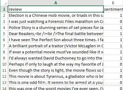

==df.reindex(np.random.permutation(df.index))==>

df.to_csv('movie_data.csv', index=False, encoding='utf-8')

df = pd.read_csv('movie_data.csv', encoding='utf-8')
df.head(3)

Processing documents into tokens

def tokenizer(text):
    return text.split()
 
from nltk.stem.porter import PorterStemmer
 
porter = PorterStemmer()
 
def tokenizer_porter(text):
    return [porter.stem(word) for word in text.split()]
 
 
import nltk
 
nltk.download('stopwords')

from nltk.corpus import stopwords
 
stop = stopwords.words('english')

continue... sklearn.feature_extraction.text.HashingVectorizer and Decomposing text documents with LDA...cp8_Sentiment_urlretrieve_pyprind_tarfile_bag词袋_walk目录_regex_verbose_pyrind_Hash_colab_verbose_文本向量化 https://blog.csdn.net/Linli522362242/article/details/110155280
##################################
Alternative method 2 : https://github.com/rasbt/python-machine-learning-book-3rd-edition/blob/master/ch08/movie_data.csv.gz

shutil.copyfileobj(fsrc, fdst[, length])

     Copy the contents of the file-like object fsrc to the file-like object fdst. The integer length, if given, is the buffer size. In particular, a negative length value means to copy the data without looping over the source data in chunks; by default the data is read in chunks to avoid uncontrolled memory consumption. Note that if the current file position of the fsrc object is not 0, only the contents from the current file position to the end of the file will be copied.

import os
import gzip
import shutil

with gzip.open('movie_data.csv.gz', 'rb') as f_in, open ('movie_data.csv', 'wb') as f_out:
    shutil.copyfileobj(f_in, f_out)

df = pd.read_csv('movie_data.csv', encoding='utf-8')

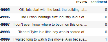
df.tail()

     Remember that this data frame, df, consists of two columns, namely 'review' and 'sentiment', where 'review' contains the text of movie reviews (the input features), and 'sentiment' represents the target label we want to predict (0 refers to negative sentiment and 1 refers to positive sentiment). The text component of these movie reviews is sequences of words, and the RNN model classifies each sequence as a positive (1) or negative (0) review.

However, before we can feed the data into an RNN model, we need to apply several preprocessing steps:
1. Create a TensorFlow dataset object and split it into separate training, testing, and validation partitions.
2. Identify the unique words in the training dataset.
3. Map each unique word to a unique integer and encode the review text into encoded integers (an index of each unique word).
4. Divide the dataset into mini-batches as input to the model.

Let's proceed with the first step: creating a TensorFlow dataset from this data frame:
#####################################################################

[ [train_string], [train_string], ... , [train_string] ] ~~~ [...target_label...]

import tensorflow as tf

# Step 1: Create a dataset

target = df.pop('sentiment') #series # key: [value_list]
ds_raw = tf.data.Dataset.from_tensor_slices(
    (df.values, # array([ [...string...], [...string...], ...]
     target.values)
)# 

## inspection:
for item in ds_raw.take(1):
    # item[0].numpy() : array([...string...])
    tf.print( item[0].numpy(), item[1] )

for item in ds_raw.take(1):
    # item[0].numpy() : array([...string...])
    tf.print( item[0].numpy()[0], item[1] )

#####################################################################

1. Create a TensorFlow dataset object and split it into separate training, testing, and validation partitions.

import tensorflow as tf

# Step 1: Create a dataset

target = df.pop('sentiment') #series # key: [value_list]
ds_raw = tf.data.Dataset.from_tensor_slices(
    (df.values, # array([ [...string...], [...string...], ...]
     target.values)
)# 

## inspection:
for item in ds_raw.take(3):
    # item[0].numpy() : array([...string...])
    tf.print( item[0].numpy()[0][:50], item[1] )

     Now, we can split it into training, testing, and validation datasets. The entire dataset contains 50,000 examples. We will keep the first 25,000 examples for evaluation (hold-out testing dataset), and then 20,000 examples will be used for training and 5,000 for validation. The code is as follows:

tf.random.set_seed(1)

ds_raw = ds_raw.shuffle(
    50000, reshuffle_each_iteration=False
) # 50000 <== 0~49999

ds_raw_test = ds_raw.take(25000)
ds_raw_train_valid = ds_raw.skip(25000)
ds_raw_train = ds_raw_train_valid.take(20000)
ds_raw_valid = ds_raw_train_valid.skip(20000)

     To prepare the (text) data for input to a NN, we need to encode it into numeric values, as was mentioned in steps 2 and 3. To do this, we will first find the unique words (tokens) in the training dataset. While finding unique tokens is a process for which we can use Python datasets, it can be more efficient to use the Counter class from the collections package, which is part of Python's standard library. (If you want to learn more about Counter, refer to its documentation at https://docs.python.org/3/library/collections.html#collections.Counter. more simpler than from sklearn.feature_extraction.text import CountVectorizer https://blog.csdn.net/Linli522362242/article/details/110155280)

     In the following code, we will instantiate a new Counter object (token_counts) that will collect the unique word frequencies.

cnt = Counter()
for word in ['red', 'blue', 'red', 'green', 'blue', 'blue']:
    cnt[word] += 1
cnt

https://docs.python.org/3/library/collections.html#collections.Counter
Note that in this particular application (and in contrast to the bag-of-words model, e.g. CountVectorizer,https://blog.csdn.net/Linli522362242/article/details/110155280

1. We create a vocabulary of unique tokens—for example, words—from the entire set of documents.

   
   import numpy as np
   from sklearn.feature_extraction.text import CountVectorizer
    
   count = CountVectorizer()
   docs = np.array([
       'The sun is shining',
       'The weather is sweet',
       'The sun is shining, the weather is sweet, and one and one is two'
   ])
    
   bag = count.fit_transform(docs)

   print( count.vocabulary_)

   # word:index 

   the vocabulary is stored in a Python dictionary that maps the unique words to integer indices.

2.  We construct a feature vector from each document that contains the counts of how often each word occurs in the particular document.

   print(bag.toarray())

   # 3 ==> 1('is', at index position 1,  occurs 3 times)

), we are only interested in the set of unique words and won't require the word counts, which are created as a side product. To split the text into words (or tokens), the tensorflow_datasets package provides a Tokenizer class.

The code for collecting unique tokens is as follows:
########################################

Tokenizer 

https://huggingface.co/transformers/main_classes/tokenizer.html

     A tokenizer is in charge of preparing the inputs for a model. The library contains tokenizers for all the models. Most of the tokenizers are available in two flavors: a full python implementation and a “Fast” implementation based on the Rust library tokenizers. The “Fast” implementations allows:

1. a significant speed-up in particular when doing batched tokenization and
2. additional methods to map between the original string (character and words) and the token space (e.g. getting the index of the token comprising a given character or the span of characters corresponding to a given token). Currently no “Fast” implementation is available for the SentencePiece-based tokenizers (for T5, ALBERT, CamemBERT, XLMRoBERTa and XLNet models).

https://www.tensorflow.org/datasets/api_docs/python/tfds/deprecated/text/Tokenizer

tfds.deprecated.text.Tokenizer

     Splits a string into tokens, and joins them back.

tfds.deprecated.text.Tokenizer(
    alphanum_only=True, reserved_tokens=None
)

• alphanum_only : bool, if True, only parse out alphanumeric字母数字 tokens (non-alphanumeric characters are dropped); otherwise, keep all characters (individual tokens will still be either all alphanumeric or all non-alphanumeric).
  Note that the Tokenizer is invertible if `alphanum_only=False`. i.e. `s == t.join(t.tokenize(s))`.  <== t =  tfds.features.text.Tokenizer()
• reserved_tokens ： list, a list of strings that, if any are in `s`, will be preserved as whole tokens, even if they contain mixed alphanumeric/non-alphanumeric characters.

tfds.features.text.Tokenizer().tokenize( text str) 

     # Splits a string into tokens.
     Converts a string in a sequence of tokens, using the tokenizer.
     Split in words for word-based vocabulary or sub-words for sub-word-based vocabularies (BPE/SentencePieces/WordPieces). Takes care of added tokens.

# Step 2: find unique tokens  (words)

from collections import Counter
import tensorflow_datasets as tfds

token_counts = Counter()
tokenizer = tfds.features.text.Tokenizer()

for example in ds_raw_train.take(1):
    print(example[0].numpy()[0][:50])
    tokens = tokenizer.tokenize(example[0].numpy()[0][:50])#numpy()[0] get first element in arr
    print(tokens)
    token_counts.update(tokens)
    print(token_counts)

print('Vocab-size:', len(token_counts))

b"okay, this movie f*ck in' rules. it is without que"                    # text string
['okay', 'this', 'movie', 'f', 'ck', 'in', 'rules', 'it', 'is', 'without', 'que']       # similar to text.split()
Counter({'okay': 1, 'this': 1, 'movie': 1, 'f': 1, 'ck': 1, 'in': 1, 'rules': 1, 'it': 1, 'is': 1, 'without': 1, 'que': 1}) #  dict ( map )
Vocab-size: 11 

tfds.deprecated.text.TokenTextEncoder

          TextEncoder backed by(由...支持的) a list of tokens.

tfds.deprecated.text.TokenTextEncoder(
    vocab_list, oov_buckets=1, oov_token='UNK', lowercase=False,
    tokenizer=None, strip_vocab=True, decode_token_separator=' '
)

 Tokenization splits on (and drops) non-alphanumeric characters with regex "\W+".  ### [\W]+ : [^A-Za-z0-9_]+

https://www.tensorflow.org/datasets/api_docs/python/tfds/deprecated/text/TokenTextEncoder

########################################

To split the text into words (or tokens)

# Step 2: find unique tokens  (words)

from collections import Counter
import tensorflow_datasets as tfds

token_counts = Counter()
tokenizer = tfds.features.text.Tokenizer()

for example in ds_raw_train:
    tokens = tokenizer.tokenize(example[0].numpy()[0])#numpy()[0] get first element in arr
    token_counts.update(tokens)

print('Vocab-size:', len(token_counts))

     Next, we are going to map each unique word(each token) to a unique integer. This can be done manually using a Python dictionary, where the keys are the unique tokens (words) and the value associated with each key is a unique integer. However, the tensorflow_datasets package already provides a class, TokenTextEncoder, which we can use to create such a mapping and encode the entire dataset.

     First, we will create an encoder object from the TokenTextEncoder class by passing the unique tokens of ds_raw_train (token_counts contains the tokens and their counts, although here, their counts are not needed, so they will be ignored). Calling the encoder.encode() method will then convert its input text into a list of integer values(IDs):

# Step 3: encoding each unique token into integers

encoder = tfds.features.text.TokenTextEncoder( token_counts )

example_str = 'This is an example!'
encoder.encode(example_str)

     Note that there might be some tokens in the validation or testing data that are not present in the training data and are thus not included in the mapping. If we have q tokens (that is the size of token_counts passed to the TokenTextEncoder, which in this case is 87,007), then all tokens that haven't been seen before, and are thus not included in token_counts, will be assigned the integer q + 1 (which will be 87,008 in our case). In other words, the index q + 1 is reserved for unknown words. Another reserved value is the integer 0, which serves as a placeholder for adjusting the sequence length. Later, when we are building an RNN model in TensorFlow, we will consider these two placeholders, 0 and q + 1, in more detail.

     We can use the map() method of the dataset objects to transform each text in the dataset accordingly, just like we would apply any other transformation to a dataset. However, there is a small problem: here, the text data is enclosed in tensor objects, which we can access by calling the numpy() method on a tensor in the eager execution mode. But during transformations by the map() method, the eager execution will be disabled. To solve this problem, we can define two functions. The first function will treat the input tensors as if the eager execution mode is enabled:

# Step 3-A: define the function for transformation

# function will treat the input tensors as if the eager execution mode is enabled
def encode(text_tensor, label):
    text = text_tensor.numpy()[0]
    encoded_text = encoder.encode(text) # encoder = tfds.features.text.TokenTextEncoder( token_counts )
    return encoded_text, label

     In the second function, we will wrap the first function using tf.py_function to convert it into a TensorFlow operator ( that executes it eagerly ), which can then be used via its map() method. This process of encoding text into a list of integers can be carried out using the following code:

# Step 3-B: wrap the encode function to a TF Op that executes it eagerly
def encode_map_fn( text, label ):
    return tf.py_function( encode, inp=[text, label],
                                  Tout=(tf.int64, tf.int64))

inp : A list of Tensor objects. https://www.tensorflow.org/api_docs/python/tf/py_function
Tout : A list or tuple of tensorflow data types or a single tensorflow data type if there is only one, indicating what func returns;
          an empty list if no value is returned (i.e., if the return value is None).

ds_train = ds_raw_train.map( encode_map_fn ) # during mapping:  the eager execution will be disabled
ds_valid = ds_raw_valid.map( encode_map_fn ) # so wrap the encode function to a TF operator that executes it eagerly
ds_test = ds_raw_test.map( encode_map_fn )

tf.random.set_seed(1)
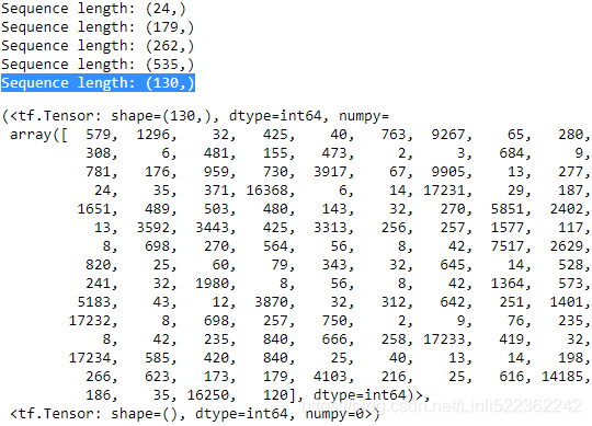
for example in ds_train.shuffle(1000).take(5):
    print('Sequence length:', example[0].shape)

example # Here, the last example's length =130, and print the IDs after doing encode

 

     So far, we've converted sequences of words into sequences of integers. However, there is one issue that we still need to resolve—the sequences currently have different lengths (as shown in the result of executing the previous code for five randomly chosen examples). Although, in general, RNNs can handle sequences with different lengths, we still need to make sure that all the sequences in a mini-batch have the same length to store them efficiently in a tensor.

     To divide a dataset that has elements with different shapes into mini-batches, TensorFlow provides a different method, padded_batch() (instead of batch()),
which will automatically pad the consecutive elements that are to be combined into a batch with placeholder values (0s) so that all sequences within a batch will have the same shape. To illustrate this with a practical example, let's take a small subset of size 8 from the training dataset, ds_train, and apply the padded_batch() method to this subset with batch_size=4. We will also print the sizes of the individual elements before combining these into mini-batches, as well as the dimensions of the resulting mini-batches:
#####################

padded_batch(
    batch_size, padded_shapes=None, padding_values=None, drop_remainder=False
)

padded_shapes : (Optional.) A nested structure of tf.TensorShape or tf.int64 vector tensor-like objects representing the shape to which the respective component of each input element should be padded prior to batching. Any unknown dimensions will be padded to the maximum size of that dimension in each batch. If unset, all dimensions of all components are padded to the maximum size in the batch. padded_shapes must be set if any component has an unknown rank.
#####################

## Take a small subset

ds_subset = ds_train.take(8) # take a small subset of size 8 from the training dataset
for example in ds_subset:
    print('Individual size:', example[0].shape)
    
## batching the datasets
ds_batched = ds_subset.padded_batch(
    4, padded_shapes=([-1], # batch_size, here is 4
                      [])   # unset, all dimensions of all components are padded to the maximum size in the batch
)

for batch in ds_batched:
    print('Batch dimension after being padded:', batch[0].shape)

Individual size: (119,)
Individual size: (688,)   #  the maximum size
Individual size: (308,)
Individual size: (204,)
Individual size: (326,)
Individual size: (240,)
Individual size: (127,)
Individual size: (453,)   # the maximum size
Batch dimension after being padded: (4, 688)
Batch dimension after being padded: (4, 453)

     As you can observe from the printed tensor shapes, the number of columns (that is, .shape[1]) in the first batch is 688, which resulted from combining the first four
examples into a single batch and using the maximum size of these examples. That means that the other three examples in this batch are padded as much as necessary to match this size. Similarly, the second batch keeps the maximum size of its individual four examples, which is 453, and pads the other examples so that their length is
smaller than the maximum length.

Let's divide all three datasets into mini-batches with a batch size of 32:

# batching the datasets
train_data = ds_train.padded_batch(
    32, padded_shapes=([-1], # batch_size, here is 32
                       [])   # unset, all dimensions of all components are padded to the maximum size in the batch
)

valid_data = ds_valid.padded_batch(
    32, padded_shapes=([-1],
                       [])
)

test_data = ds_test.padded_batch(
    32, padded_shapes=([-1],
                       [])
)

     Now, the data is in a suitable format for an RNN model, which we are going to implement in the following subsections. In the next subsection, however, we will
first discuss feature embedding, which is an optional but highly recommended preprocessing step that is used for reducing the dimensionality of the word vectors.

Embedding layers for sentence encoding

     During the data preparation in the previous step, we generated sequences of the same length( the number of feature_columns ). The elements of these sequences were integer numbers that corresponded to the indices of unique words. These word indices can be converted into input features in several different ways. One naive way is to apply one-hot(######https://blog.csdn.net/Linli522362242/article/details/108108665

simple_example = tf.constant([ [1,3,1,0,0], 
                               [2,2,0,0,0] ])
tf.one_hot(simple_example, 4)

2 sentences, each one has 5 words(the number of our input features, one input is a sentence), size=4( is the number of unique words in the entire dataset OR the size of the vocabulary)

######) encoding to convert the indices into vectors of zeros(0 if not exists) and ones(1 if exists). Then, each word will be mapped to a vector whose size is the number of unique words in the entire dataset. Given that the number of unique words (the size of the vocabulary) can be in the order of , which will also be the number of our input features, a model trained on such features may suffer from the curse of dimensionality. Furthermore, these features are very sparse, since all are zero except one.

     A more elegant approach is to map each word to a vector of a fixed size with realvalued elements (not necessarily integers). In contrast to the one-hot encoded vectors, we can use finite-sized vectors to represent an infinite number of real numbers. (In theory, we can extract infinite real numbers from a given interval, for example [–1, 1].)

     This is the idea behind embedding, which is a feature-learning technique that we can utilize here to automatically learn the salient显着的 features to represent the words in our dataset. Given the number of unique words, , we can select the size of the embedding vectors (a.k.a., embedding dimension, embedding features, and embedding_dim is the size of the embedding features, the number of embedding columns ) to be much smaller than the number of unique words ( embedding_dim << ) to represent the entire vocabulary as input features.

The advantages of embedding over one-hot encoding are as follows:

• • A reduction in the dimensionality of the feature space to decrease the effect of the curse of dimensionality
• • The extraction of salient features since the embedding layer in an NN can be optimized (or learned)

     The following schematic representation shows how embedding works by mapping token indices to a trainable embedding matrix:

13_Loading & Preproces Data from multiple CSV with TF 2_Feature Columns_TF eXtended_num_oov_bucketshttps://blog.csdn.net/Linli522362242/article/details/107933572
     Given a set of tokens of size n + 2 (==len(vocab)+num_oov_buckets, n is the size of the token set, plus index 0 is reserved for the padding placeholder, and n + 1 is for the words not present in the token set), an embedding matrix of embedding_dim x  size ( + 2) will be created where each row of this matrix represents numeric features associated with a token. Therefore, when an integer index, i, is given as input to the embedding, it will look up the corresponding row of the matrix at index i (the index of the unique words except 0 and n+1) and return the numeric features(shape=embedding_dim). The embedding matrix serves as the input layer to our NN models. In practice, creating an embedding layer can simply be done using tf.keras. layers.Embedding. Let's see an example where we will create a model and add an embedding layer, as follows:

from tensorflow.keras.layers import Embedding

model = tf.keras.Sequential()       
                                    # input_dim corresponds to the unique integer values that the model will receive  
model.add( Embedding(input_dim=100, # as input (for instance, n + 2, set here to 100; and n is number of unique words) 
                     output_dim=6,    # embedding_dim is the size of the embedding features
                     input_length=20, # input features e.g. (14, 43, 52, 61, 8,19,67,83,10,7,42,87,56,18,94,17,67,90,6,39)
                     name='embed-layer')
         )
model.summary()

     The input to this model (embedding layer) must have rank 2 with dimensionality batchsize × input_length , where input_length is the length of sequences (here,
set to 20 via the input_length argument, or input_features, or input columns). For example, an input sequence in the mini-batch could be 〈14, 43, 52, 61, 8,19,67,83,10,7,42,87,56,18,94,17,67,90,6,39〉 , where each element of this sequence is the index of the unique words. The output will have dimensionality batchsize × input_length x embedding_dim, where embedding_dim is the size of the embedding features (here, set to 6 via output_dim). The other argument provided to the embedding layer, input_dim, corresponds to the unique integer values that the model will receive as input (for instance, n + 2, set here to 100, note n is number of unique words, 2 is num_oov_buckets). Therefore, the embedding matrix in this case has the size 6 x100 .
####################

Dealing with variable sequence lengths

     Note that the input_length(input_features) argument is not required, and we can use None for cases where the lengths of input sequences vary. You can find more information about this function in the official documentation at https://www.tensorflow.org/versions/r2.0/api_docs/python/tf/keras/layers/Embedding.

Length of input sequences, when it is constant. This argument is required if you are going to connect Flatten then Dense layers upstream (without it, the shape of the dense outputs cannot be computed).

####################

Building an RNN model

     Now we're ready to build an RNN model. Using the Keras Sequential class, we can combine the embedding layer, the recurrent layers of the RNN, and the fully
connected non-recurrent layers. For the recurrent layers, we can use any of the following implementations:

• Keras RNN layers:

  • tf.keras.layers.SimpleRNN(units, return_sequences=False): a regular RNN layer, that is, a fully connected recurrent layer
  • tf.keras.layers.LSTM(..) : a long short-term memory RNN, which is useful for capturing the long-term dependencies
  • tf.keras.layers.GRU(..) : a recurrent layer with a gated recurrent unit, as proposed in Learning Phrase Representations Using RNN Encoder–Decoder for Statistical Machine Translation (https://arxiv.org/abs/1406.1078v3), as an alternative to LSTMs
  • tf.keras.layers.Bidirectional()

• Determine return_sequenes=?

  • In a multi-layer RNN, all RNN layers except the last one should have return_sequenes=True
  • For the last RNN layer, decide based on the type of problem:
    • many-to-many: -> return_sequences=True
    • many-to-one : -> return_sequenes=False
    • ..

     To see how a multilayer RNN model can be built using one of these recurrent layers, in the following example, we will create an RNN model, starting with an embedding layer with input_dim=1000 and output_dim=32 (tensorflow.keras.layers.Embedding). Then, two recurrent layers of type SimpleRNN will be added. Finally, we will add a non-recurrent fully connected layer as the output layer, which will return a single output value as the prediction:

An example of building a RNN model with SimpleRNN layer

from tensorflow.keras import Sequential
from tensorflow.keras.layers import Embedding
from tensorflow.keras.layers import SimpleRNN
from tensorflow.keras.layers import Dense

model = Sequential()
model.add(Embedding(input_dim=1000, output_dim=32))#1000=n+2=len(vocabulary)+num_oov_buckets; 32=embedding_dim=embedding features
model.add(SimpleRNN(32, return_sequences=True)) # many-to-many # 32 units : Positive integer, dimensionality of the output space.
model.add(SimpleRNN(32)) # return_sequenes=False # many-to-one
model.add( Dense(1) ) # a fully connected (FC) layer or linear layer, f(w*x=b), f is the activation function
model.summary()

An example of building a RNN model with LSTM layer

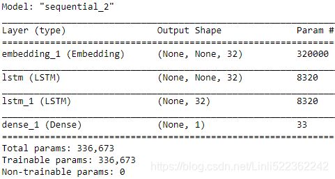
from tensorflow.keras.layers import LSTM

model = Sequential()
model.add( Embedding(10000,32) )
model.add( LSTM(32, return_sequences=True) )
model.add( LSTM(32) )
model.add( Dense(1) )# a fully connected (FC) layer or linear layer, f(w*x=b), f is the activation function

model.summary()

  

An example of building a RNN model with GRU (gated recurrent units) layer

GRU cells

     The Gated Recurrent Unit (GRU) cell (see Figure 15-10) was proposed by Kyunghyun Cho et al. in a 2014 paper_11 that also introduced the Encoder–Decoder network we
discussed earlier

     The GRU cell is a simplified version of the LSTM cell, and it seems to perform just as well(which explains its growing popularity, A 2015 paper by Klaus Greff et al., “LSTM: A Search Space Odyssey[ˈɑdɪsi]漫游”, seems to show that all LSTM variants perform roughly the same.). These are the main simplifications:

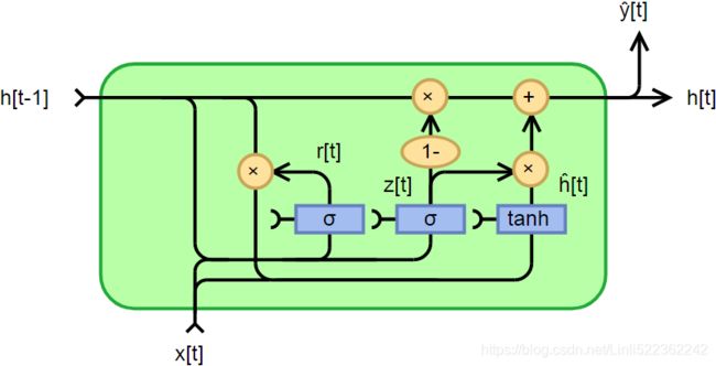
Gated Recurrent Unit, fully gated version                                          https://en.wikipedia.org/wiki/Gated_recurrent_unit
     Fully gated unit
    Initially, for t=0 , the output vector is =0.
Figure 15-10. GRU cell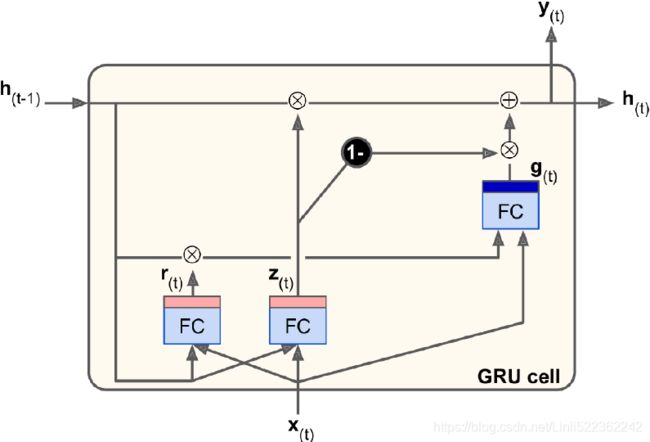 
==
                        ==
Variables : The original is a sigmoid function. and : The original is a hyperbolic tangent.

• : input vector
• : output vector
• : update gate vector ( <== input <== and  hidden: bias )
• : reset gate vector    ( <== input <== and  hidden: bias)
• OR: candidate activation vector ( <== input <==,  and )
• W, U and b: parameter matrices and vector

Activation functions
     Alternative activation functions are possible, provided that .

Left Figure:

• • Both state vectors(and ) are merged into a single vector .
• • A single gate(update gate) controller controls both the forget gate and the input gate.
       If the gate controller outputs a 1, the forget gate is open (= 1, then ) and the input gate is closed (1 – 1 = 0).
       If it outputs a 0, the opposite happens.
  In other words, whenever a memory must be stored, the location where it will be stored is erased first. This is actually a frequent variant to the LSTM cell in and of itself.
• • There is no output gate; the full state vector is output at every time step. However, there is a new gate controller (reset gate) that controls which part of the previous state will be shown to the main layer ().

Right Figure:

Alternate forms can be created by changing  and 

• Type 1, each gate depends only on the previous hidden state and the bias.
  ( <== input  and bias)
  
• Type 2, each gate depends only on the previous hidden state.
  ( <== input )
  
• Type 3, each gate is computed using only the bias.
  

Minimal gated unit

     The minimal gated unit is similar to the fully gated unit, except the update and reset gate vector is merged into a forget gate. This also implies that the equation for the output vector must be changed:
is similar to the fully gated unit

• : input vector
• : output vector
• :  forget vector( <== input <== and  hidden: bias )
• OR: candidate activation vector ( <== input <==,  and )
• W, U and b: parameter matrices and vector

     As you can see, building an RNN model using these recurrent layers is pretty straightforward. In the next subsection, we will go back to our sentiment analysis
task and build an RNN model to solve that.

Building an RNN model for the sentiment analysis task

https://blog.csdn.net/Linli522362242/article/details/114239076