强化学习-赵世钰（二）：贝尔曼/Bellman方程【用于计算给定π下的State Value：①线性方程组法、②迭代法】、Action Value【根据状态值求解得到；用来评价action优劣】

State Value ：the average Return that an agent can obtain if it follows a given policy/π【给定一个policy/π，所有可能的trajectorys得到的所有return的平均值/期望值：$v_{\pi }(s)\doteq \mathbb{E}[G_t|S_t=s]$】.
Return：the discounted sum of all the rewards collected along a trajectory【return 等于沿着一个特定的 trajectory 收集到的所有 rewards 的折现总和：$G_t\doteq R_{t+1}+\gamma R_{t+2}+{\gamma }^2{R}_{t+3}+\dots ,$】

$v_{\pi }(s)$：从状态 $s$ 出发，遵循策略 $\pi$ 能够获得的期望回报。

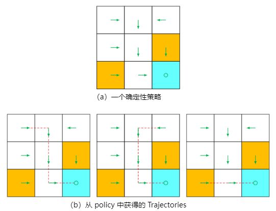
• 从给定状态 $s_i$ 出发基于给定的policy/π所包含的trajectorys之所以有多个，是因为在每个state时agent接下来要采取的action是按该policy下的概率来采样的，如下图：
  如果每一个state处所采取的action是固定的（以箭头表示），则每一个state在该policy中只有一个固定的trajectory；
  

• $v_{\pi }(s)$ depends on $s$：This is because its defnition is a conditional expectation with the condition that the agent starts from $S_t=s.$

• $v_{\pi }(s)$ depends on $\pi$：This is because the trajectories are generated by following the policy $\pi$. For a different policy, the state value may be different.【不同的policy/π得到的trajectories集合是不一样的】

• $v_{\pi }(s)$ does not depend on $t$：If the agent moves in the state space, $t$ represents the current time step. The value of ${\upsilon }_{\pi }(s)$ is determined once the policy is given.

state values和returns之间的关系进一步明确如下：

• When both the policy and the system model are deterministic, starting from a state always leads to the same trajectory. In this case, the return obtained starting from a state is equal to the value of that state. 【当 policy 和 system model 都是确定性的时候，从一个状态开始总是会导致相同的轨迹。在这种情况下，从一个状态开始获得的return等于该状态的state value】
• By contrast, when either the policy or the system model is stochastic, starting from the same state may generate different trajectories. In this case, the returns of different trajectories are different, and the state value is the mean of these returns.【相反，当 policy 或 system model 中的任何一个是随机的时候，从相同的 state 开始可能会产生不同的trajectory。在这种情况下，不同trajectory的return是不同的，而state value是这些return的平均值。】
• The greater the state value is, the better the corresponding policy is.
• State values can be used as a metric to evaluate whether a policy is good or not.

While state values are important, how can we analyze them?

• The answer is the Bellman equation（贝尔曼方程）, which is an important tool for analyzing state values.
• In a nutshell, the Bellman equation describes the relationships between the values of all states.【贝尔曼方程描述了所有状态值之间的关系。】
• By solving the Bellman equation, we can obtain the state values. This process is called policy evaluation, which is a fundamental concept in reinforcement learning. 【通过解决贝尔曼方程，我们可以得到状态值。这个过程被称为策略评估，是强化学习中的基本概念。】

Finally, this chapter introduces another important concept called the action value.

2.1 Motivating example 1: Why are returns important?

The previous chapter introduced the concept of returns. In fact, returns play a fundamental role in reinforcement learning since they can evaluate whether a policy is good or not. This is demonstrated by the following examples.

Consider the three policies shown in Figure 2.2. It can be seen that the three policies are different at s1. Which is the best and which is the worst? Intuitively,

• the leftmost policy is the best because the agent starting from $s_1$ can avoid the forbidden area. 【最左边的策略是最好的，因为从$s_1$开始的agent可以避开禁区】
• The middle policy is intuitively worse because the agent starting from $s_1$ moves to the forbidden area. 【中间的策略直观上更差，因为从$s_1$开始的agent会移动到禁区】
• The rightmost policy is in between the others because it has a probability of 0.5 to go to the forbidden area.【最右边的策略介于其他两者之间，因为它 有0.5的概率进入禁区】

While the above analysis is based on intuition, a question that immediately follows is whether we can use mathematics to describe such intuition. The answer is yes and relies on the return concept. 【尽管上述分析是基于直觉的，但紧随其后的一个问题是我们是否可以使用数学来描述这种直觉。答案是肯定的，这依赖于return的概念】

In particular, suppose that the agent starts from $s_1$.

• Following the first policy, the trajectory is s1 → s3 → s4 → s4 · · · . The corresponding discounted return is
  $$\begin{array}{rl}retur{n}_1& =0+\gamma 1+{\gamma }^{2}1+\dots \\ & =\gamma (1+\gamma +{\gamma }^2+\dots )\\ & =\frac{\gamma }{1-\gamma },\end{array}$$
  where $\gamma \in (0,1)$ is the discount rate.
• Following the second policy, the trajectory is s1 → s2 → s4 → s4 · · · . The discounted return is

$$\begin{array}{rl}retur{n}_2& \begin{array}{r}=-1+\gamma 1+{\gamma }^{2}1+\dots \end{array}\\ & =-1+\gamma (1+\gamma +{\gamma }^2+\dots )\\ & =-1+\frac{\gamma }{1-\gamma }.\end{array}$$

• Following the third policy, two trajectories can possibly be obtained. One is s1 → s3 → s4 → s4 · · · , and the other is s1 → s2 → s4 → s4 · · · . The probability of either of the two trajectories is 0.5. Then, the average return that can be obtained starting from $s_1$ is

$$\begin{array}{rl}retur{n}_3& \begin{array}{r}=0.5\left(-1+\frac{\gamma }{1-\gamma }\right)+0.5\left(\frac{\gamma }{1-\gamma }\right)\end{array}\\ & =-0.5+\frac{\gamma }{1-\gamma }.\end{array}$$

By comparing the returns of the three policies, we notice that：
$$retur{n}_1>retur{n}_3>retur{n}_2$$

for any value of γ. $retur{n}_1>retur{n}_3>retur{n}_2$ suggests that the first policy is the best because its return is the greatest, and the second policy is the worst because its return is the smallest.

This mathematical conclusion is consistent with the aforementioned intuition: the first policy is the best since it can avoid entering the forbidden area, and the second policy is the worst because it leads to the forbidden area.

2.2 Motivating example 2: How to calculate returns?

While we have demonstrated the importance of returns, a question that immediately follows is how to calculate the returns when following a given policy.

There are two ways to calculate returns. 【有两种计算return的方法】

• The first is simply by definition: a return equals the discounted sum of all the rewards collected along a trajectory【return 等于沿着一个 trajectory 收集到的所有奖励的折现总和】. Consider the example in Figure 2.3. Let $v_i$ denote the return obtained by starting from $s_i$ for i = 1, 2, 3, 4. Then, the returns obtained when starting from the four states in Figure 2.3 can be calculated as
  
• The second way, which is more important, is based on the idea of bootstrapping. By observing the expressions of the returns in (2.2), we can rewrite them as
  
  The above equations indicate an interesting phenomenon that the values of the returns rely on each other. More specifically, v1 relies on v2, v2 relies on v3, v3 relies on v4, and v4 relies on v1. This reflects the idea of bootstrapping, which is to obtain the values of some quantities from themselves.

At first glance, bootstrapping is an endless loop because the calculation of an unknown value relies on another unknown value. In fact, bootstrapping is easier to understand if we view it from a mathematical perspective. In particular, the equations in (2.3) can be reformed into a linear matrix-vector equation:

which can be written compactly as
$$v=r+\gamma Pv.$$
Thus, the value of $v$ can be calculated easily as $v=(I-\gamma P{)}^{-1}r$, where $I$ is the identity matrix with appropriate dimensions. One may ask whether $I-\gamma P$ is always invertible. The answer is yes and explained in Section 2.7.1.

In fact, (2.3) is the Bellman equation for this simple example. Although it is simple, (2.3) demonstrates the core idea of the Bellman equation: the return obtained by starting from one state depends on those obtained when starting from other states.

2.3 State values

We mentioned that returns can be used to evaluate policies. However, they are inapplicable to stochastic systems because starting from one state may lead to different returns.【我们提到过returns可以用来评估policies。然而，在随机系统中，returns是不适用的，因为从一个state出发可能会导致不同的returns】

Motivated by this problem, we introduce the concept of state value in this section.

First, we need to introduce some necessary notations.

Consider a sequence of time steps $t=0,1,2,\dots$ At time $t$, the agent is at state $S_t$, and the action taken following a policy $\pi$ is $A_t.$ The next state is $S_{t+1}$, and the immediate reward obtained is $R_{t+1}.$ This process can be expressed concisely as

$$S_t\stackrel{A_t}{}{S}_{t+1},R_{t+1}$$

Note that $S_t,S_{t+1},A_t,R_{t+1}$ are all random variables. Moreover, $S_t,S_{t+1}\in \mathcal{S},A_t\in \mathcal{A}(S_t)$, and $R_{t+1}\in \mathcal{R}(S_t,A_t)$.

Starting from $t$, we can obtain a state-action-reward trajectory:

$$\begin{array}{r}{S}_t\stackrel{A_t}{}{S}_{t+1},R_{t+1}\stackrel{A_{t+1}}{}{S}_{t+2},R_{t+2}\stackrel{A_{t+2}}{}{S}_{t+3},R_{t+3}\dots .\end{array}$$

By definition, the discounted return along the trajectory【注：在给定π条件下，可能有多个trajectory】 is
$$G_t\doteq R_{t+1}+\gamma R_{t+2}+{\gamma }^2{R}_{t+3}+\dots ,$$
where γ ∈ (0, 1) is the discount rate. Note that Gt is a random variable since $\begin{array}{r}{R}_{t+1},R_{t+2},\dots \end{array}$ are all random variables.

Since $G_t$ is a random variable, we can calculate its expected value (also called the expectation or mean):

$$v_{\pi }(s)\doteq \mathbb{E}[G_t|S_t=s]$$

Here, $v_{\pi }(s)$ is called the state-value function or simply the state value of s.

Some important remarks are given below.

• $v_{\pi }(s)$ depends on $s$：This is because its defnition is a conditional expectation with the condition that the agent starts from $S_t=s.$
• $v_{\pi }(s)$ depends on $\pi$：This is because the trajectories are generated by following the policy $\pi$. For a different policy, the state value may be different.【不同的policy/π得到的trajectories集合是不一样的】
• $v_{\pi }(s)$ does not depend on $t$：If the agent moves in the state space, $t$ represents the current time step. The value of ${\upsilon }_{\pi }(s)$ is determined once the policy is given.

state values和returns之间的关系进一步明确如下：

• When both the policy and the system model are deterministic, starting from a state always leads to the same trajectory. In this case, the return obtained starting from a state is equal to the value of that state. 【当 policy 和 system model 都是确定性的时候，从一个状态开始总是会导致相同的轨迹。在这种情况下，从一个状态开始获得的return等于该状态的state value】
• By contrast, when either the policy or the system model is stochastic, starting from the same state may generate different trajectories. In this case, the returns of different trajectories are different, and the state value is the mean of these returns.【相反，当 policy 或 system model 中的任何一个是随机的时候，从相同的 state 开始可能会产生不同的trajectory。在这种情况下，不同trajectory的return是不同的，而state value是这些return的平均值。】

2.4 Bellman equation【贝尔曼公式】

Bellman equation, a mathematical tool for analyzing state val- ues. In a nutshell, the Bellman equation is a set of linear equations that describe the relationships between the values of all the states.【贝尔曼方程，这是一种分析状态值的数学工具。简而言之，贝尔曼方程是一组线性方程，描述了所有状态值之间的关系。】

贝尔曼公式推导：

• First, note that $G_t$ can be rewritten as
  $$\begin{array}{rl}{G}_t& \begin{array}{r}=R_{t+1}+\gamma R_{t+2}+{\gamma }^2{R}_{t+3}+\dots \end{array}\\ & =R_{t+1}+\gamma (R_{t+2}+\gamma R_{t+3}+\dots )\\ & =R_{t+1}+\gamma G_{t+1}\end{array}$$

where $\begin{array}{r}{G}_{t+1}=R_{t+2}+\gamma R_{t+3}+\dots .\end{array}$ This equation establishes the relationship between $G_t$ and $G_{t+1}$.

State Value 表示为(2.4) ：
$$\begin{array}{rl}{\upsilon }_{\pi }(s)& =\mathbb{E}[G_t|S_t=s]\\ & =\mathbb{E}[R_{t+1}+\gamma G_{t+1}|S_t=s]\\ & =\mathbb{E}[R_{t+1}|S_t=s]+\gamma \mathbb{E}[G_{t+1}|S_t=s]\end{array}$$

• 第一项 $\mathbb{E}[R_{t+1}|S_t=s]$ 表示 the expectation of immediate rewards，根据the law of total expectation，可被改写为(2.5)：
  $$\begin{array}{rl}\mathbb{E}[R_{t+1}|S_t=s]& =\sum _{a\in \mathcal{A}}\pi (a|s)\mathbb{E}[R_{t+1}|S_t=s,A_t=a]\\ & =\sum _{a\in \mathcal{A}}\pi (a|s)\sum _{r\in \mathcal{R}}p(r|s,a)r\end{array}$$
  • Here, $A$ and $R$ are the sets of possible actions and rewards, respectively.
  • It should be noted that A may be different for different states.
  • In this case, $A$ should be written as $A(s)$. Similarly, $R$ may also depend on $(s,a)$.
  • We drop the dependence on $s$ or $(s,a)$ for the sake of simplicity in this book. 【为了书写简洁】
  • Nevertheless, the conclusions are still valid in the presence of dependence.
• 第二项 $\mathbb{E}[G_{t+1}|S_t=s]$ ,表示 the expectation of the future rewards，可被改写为：
  $$\begin{array}{rl}\mathbb{E}[G_{t+1}|S_t=s]& =\sum _{s^{\prime }\in \mathcal{S}}\mathbb{E}[G_{t+1}|S_t=s,S_{t+1}=s^{\prime }]p(s^{\prime }|s)\\ & =\sum _{s^{\prime }\in \mathcal{S}}\mathbb{E}[G_{t+1}|S_{t+1}=s^{\prime }]p(s^{\prime }|s)\text{(due to the Markov property)}\\ & =\sum _{s^{\prime }\in \mathcal{S}}{v}_{\pi }(s^{\prime })p(s^{\prime }|s)\\ & =\sum _{s^{\prime }\in \mathcal{S}}{v}_{\pi }(s^{\prime })\sum _{a\in \mathcal{A}}p(s^{\prime }|s,a)\pi (a|s)\end{array}$$
  • The above derivation uses the fact that $\mathbb{E}[G_{t+1}|S_t=s,S_{t+1}=s^{\prime }]=\mathbb{E}[G_{t+1}|S_{t+1}=s^{\prime }]$，which is due to the Markov property that the future rewards depend merely on the present state rather than the previous ones.
  • $s^{\prime }$ 表示 $s$ 的下一个时刻的状态；

将(2.5)-(2.6)代入(2.4)，得公式(2.7)：

$$\begin{array}{rl}{v}_{\pi }(s)& =\mathbb{E}[R_{t+1}|S_t=s]+\gamma \mathbb{E}[G_{t+1}|S_t=s]\\ & =\underset{\text{mean of immediate rewards}}{\sum _{a\in \mathcal{A}}\pi (a|s)\sum _{r\in \mathcal{R}}p(r|s,a)r}+\underset{\text{mean of future rewards}}{\gamma \sum _{a\in \mathcal{A}}\pi (a|s)\sum _{s^{\prime }\in \mathcal{S}}p(s^{\prime }|s,a)v_{\pi }(s^{\prime }),}\\ & =\sum _{a\in \mathcal{A}}\pi (a|s)\left[\sum _{r\in \mathcal{R}}p(r|s,a)r+\gamma \sum _{s^{\prime }\in \mathcal{S}}p(s^{\prime }|s,a)v_{\pi }(s^{\prime })\right],\text{for all }s\in \mathcal{S}\end{array}$$

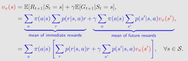
This equation is the Bellman equation, which characterizes the relationships of state values. It is a fundamental tool for designing and analyzing reinforcement learning algorithms.【这个方程是贝尔曼方程，它描述了state value之间的关系。它是设计和分析强化学习算法的基本工具。】

• $v_{\pi }(s)$ and $v_{\pi }(s^{\prime })$ are unknown state values to be calculated.
  • the Bellman equation refers to a set of linear equations for all states rather than a single equation.
  • If we put these equations together, it becomes clear how to calculate all the state values.
• $\pi (a|s)$ is a given policy.
  • Since state values can be used to evaluate a policy, solving the state values from the Bellman equation is a $policyevaluation$ process.
• $p(r|s,a)$ and $p(s^{\prime }|s,a)$ represent the system model.
  • We will first show how to calculate the state values $with$ this model and then show how to do that $without$ the model by using model-free algorithms later in this book.

In addition to the expression in (2.7), readers may also encounter other expressions of the Bellman equation in the literature. We next introduce two equivalent expressions.

• First, it follows from the law of total probability that
  $$\begin{array}{rl}p(s^{\prime }|s,a)& =\sum _{r\in \mathcal{R}}p(s^{\prime },r|s,a),\\ p(r|s,a)& =\sum _{s^{\prime }\in \mathcal{S}}p(s^{\prime },r|s,a).\end{array}$$
  Then, equation (2.7) can be rewritten as
  $$\begin{array}{r}{v}_{\pi }(s)=\sum _{a\in \mathcal{A}}\pi (a|s)\sum _{s^{\prime }\in \mathcal{S}}\sum _{r\in \mathcal{R}}p(s^{\prime },r|s,a)\left[r+\gamma v_{\pi }(s^{\prime })\right]\end{array}$$
• Second, the reward $r$ may depend solely on the next state $s^{\prime }$ in some problems. As a result, we can write the reward as $r(s^{\prime })$ and hence $p(r(s^{\prime })|s,a)=p(s^{\prime }|s,a)$, substituting which into (2.7) gives
  $$\begin{array}{rl}{v}_{\pi }(s)& =\sum _{a\in \mathcal{A}}\pi (a|s)\sum _{s^{\prime }\in \mathcal{S}}p(s^{\prime }|s,a)\left[r(s^{\prime })+\gamma v_{\pi }(s^{\prime })\right]\end{array}$$

2.5 Examples for illustrating the Bellman equation

We next use two examples to demonstrate how to write out the Bellman equation and calculate the state values step by step. Readers are advised to carefully go through the examples to gain a better understanding of the Bellman equation.【我们接下来使用两个例子来演示如何写出贝尔曼方程并逐步计算状态值。建议读者仔细阅读这些例子，以更好地理解贝尔曼方程。】

If we compare the state values of the two policies in the above examples, it can be seen that：【如果我们比较下述示例中两种策略的状态值，可以看到】
$$v_{{\pi }_1}(s_i)\ge v_{{\pi }_2}(s_i),i=1,2,3,4,$$

• which indicates that the policy in Figure 2.4 is better because it has greater state values.【这表明图2.4中的策略更好，因为它具有更大的状态值。】
• This mathematical conclusion is consistent with the intuition that the first policy is better because it can avoid entering the forbidden area when the agent starts from $s_1$. 【这个数学结论与直觉一致，即第一个policy更好，因为当agent 从$s_1$开始时，它可以避免进入禁区。】
• As a result, the above two examples demonstrate that state values can be used to evaluate policies.【这两个例子证明了state value可以 用来评估policy】

2.5.1 example01【policy是确定性的】

Consider the first example shown in Figure 2.4, where the policy is deterministic【policy是确定性的】.

We next write out the Bellman equation and then solve the state values from it.

First, consider state $s_1.$ Under the policy：

• The probabilities of taking the actions are $\pi (a=a_3|s_1)=1$ and $\pi (a\ne a_3|s_1)=0$.
• The state transition probabilities are $p(s^{\prime }=s_3|s_1,a_3)=1$ and $p(s^{\prime }\ne s_3|s_1,a_3)=0.$
• The reward probabilities are $p(r=0|s_1,a_3)=1$ and $p(r\ne 0|s_1,a_3)=0.$

Substituting these values into
$$\begin{array}{rl}{v}_{\pi }(s)& =\mathbb{E}[R_{t+1}|S_t=s]+\gamma \mathbb{E}[G_{t+1}|S_t=s]\\ & =\underset{\text{mean of immediate rewards}}{\sum _{a\in \mathcal{A}}\pi (a|s)\sum _{r\in \mathcal{R}}p(r|s,a)r}+\underset{\text{mean of future rewards}}{\gamma \sum _{a\in \mathcal{A}}\pi (a|s)\sum _{s^{\prime }\in \mathcal{S}}p(s^{\prime }|s,a)v_{\pi }(s^{\prime }),}\\ & =\sum _{a\in \mathcal{A}}\pi (a|s)\left[\sum _{r\in \mathcal{R}}p(r|s,a)r+\gamma \sum _{s^{\prime }\in \mathcal{S}}p(s^{\prime }|s,a)v_{\pi }(s^{\prime })\right],\text{for all }s\in \mathcal{S}\end{array}$$

gives
$$v_{\pi }(s_1)=0+\gamma v_{\pi }(s_3)$$

Similarly, it can be obtained that
$$\begin{array}{rl}& {\upsilon }_{\pi }(s_2)=1+\gamma {\upsilon }_{\pi }(s_4)\\ & v_{\pi }(s_3)=1+\gamma {\upsilon }_{\pi }(s_4)\\ & {\upsilon }_{\pi }(s_4)=1+\gamma {\upsilon }_{\pi }(s_4)\end{array}$$

We can solve the state values from these equations. Since the equations are simple, we can manually solve them. Here, the state values can be solved as：【我们可以从这些方程中解出状态值。由于这些方程很简单，我们可以手动解决它们。在这里，状态值可以被解决为】
$$\begin{array}{c}{\upsilon }_{\pi }(s_4)=\frac{1}{1-\gamma },\\ {\upsilon }_{\pi }(s_3)=\frac{1}{1-\gamma },\\ {\upsilon }_{\pi }(s_2)=\frac{1}{1-\gamma },\\ {\upsilon }_{\pi }(s_1)=\frac{\gamma }{1-\gamma }.\end{array}$$

Furthermore, if we set $\gamma =0.9$, then
$$\begin{array}{c}{\upsilon }_{\pi }(s_4)\begin{array}{r}=\frac{1}{1-0.9}=10,\end{array}\\ {\upsilon }_{\pi }(s_3)=\frac{1}{1-0.9}=10,\\ {\upsilon }_{\pi }(s_2)=\frac{1}{1-0.9}=10,\\ {\upsilon }_{\pi }(s_1)=\frac{0.9}{1-0.9}=9.\end{array}$$

2.5.2 example02【policy是随机的】

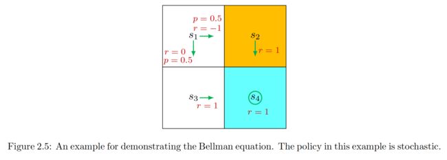
Consider the second example shown in Figure 2.5, where the policy is stochastic【policy是随机的】.

We next write out the Bellman equation and then solve the state values from it.

First, consider state $s_1.$ Under the policy：

• At state $s_1$, the probabilities of going right and down equal 0.5. The probabilities of taking the actions are $\pi (a=a_2|s_1)=0.5$ and $\pi (a=a_3|s_1)=\mathrm{0.5.}$
• The state transition probability is deterministic since $p(s^{\prime }=s_3|s_1,a_3)=1$ and $p(s^{\prime }=s_2|s_1,a_2)=1.$
• The reward probability is also deterministic since $p(r=0|s_1,a_3)=1$ and $p(r=-1|s_1,a_2)=1.$

Substituting these values into
$$\begin{array}{rl}{v}_{\pi }(s)& =\mathbb{E}[R_{t+1}|S_t=s]+\gamma \mathbb{E}[G_{t+1}|S_t=s]\\ & =\underset{\text{mean of immediate rewards}}{\sum _{a\in \mathcal{A}}\pi (a|s)\sum _{r\in \mathcal{R}}p(r|s,a)r}+\underset{\text{mean of future rewards}}{\gamma \sum _{a\in \mathcal{A}}\pi (a|s)\sum _{s^{\prime }\in \mathcal{S}}p(s^{\prime }|s,a)v_{\pi }(s^{\prime }),}\\ & =\sum _{a\in \mathcal{A}}\pi (a|s)\left[\sum _{r\in \mathcal{R}}p(r|s,a)r+\gamma \sum _{s^{\prime }\in \mathcal{S}}p(s^{\prime }|s,a)v_{\pi }(s^{\prime })\right],\text{for all }s\in \mathcal{S}\end{array}$$

gives
$$\begin{array}{r}{v}_{\pi }(s_1)=0.5[0+\gamma v_{\pi }(s_3)]+0.5[-1+\gamma v_{\pi }(s_2)]\end{array}$$

Similarly, it can be obtained that

$$\begin{array}{rl}& {\upsilon }_{\pi }(s_2)=1+\gamma {\upsilon }_{\pi }(s_4),\\ & {\upsilon }_{\pi }(s_3)=1+\gamma {\upsilon }_{\pi }(s_4),\\ & {\upsilon }_{\pi }(s_4)=1+\gamma {\upsilon }_{\pi }(s_4).\end{array}$$

The state values can be solved from the above equations. Since the equations are simple, we can solve the state values manually and obtain

$$\begin{array}{rl}& v_{\pi }(s_4)=\frac{1}{1-\gamma },\\ & {\upsilon }_{\pi }(s_3)=\frac{1}{1-\gamma },\\ & {\upsilon }_{\pi }(s_2)=\frac{1}{1-\gamma },\\ & v_{\pi }(s_1)=0.5[0+\gamma v_{\pi }(s_3)]+0.5[-1+\gamma v_{\pi }(s_2)]=-0.5+\frac{\gamma }{1-\gamma }\end{array}$$

Furthermore, if we set $\gamma =0.9$, then

$$\begin{array}{rl}& {\upsilon }_{\pi }(s_4)=10,\\ & {\upsilon }_{\pi }(s_3)=10,\\ & v_{\pi }(s_2)=10,\\ & v_{\pi }(s_1)=-0.5+9=\mathrm{8.5.}\end{array}$$

2.6 Matrix-vector form of the Bellman equation【贝尔曼方程的矩阵-向量形式】

The Bellman equation in (2.7) is in an element-wise form. Since it is valid for every state, we can combine all these equations and write them concisely in a matrix-vector form, which will be frequently used to analyze the Bellman equation.【贝尔曼方程(2.7)是以元素形式表示的。由于它对于每个状态都有效，我们可以将所有这些方程组合起来，并以矩阵-向量形式简洁地写出来，将经常用于分析贝尔曼方程。】

To derive the matrix-vector form, we first rewrite the Bellman equation【为了得到矩阵-向量形式，我们首先将贝尔曼方程重写】

$$\begin{array}{rl}{v}_{\pi }(s)& =\mathbb{E}[R_{t+1}|S_t=s]+\gamma \mathbb{E}[G_{t+1}|S_t=s]\\ & =\underset{\text{mean of immediate rewards}}{\sum _{a\in \mathcal{A}}\pi (a|s)\sum _{r\in \mathcal{R}}p(r|s,a)r}+\underset{\text{mean of future rewards}}{\gamma \sum _{a\in \mathcal{A}}\pi (a|s)\sum _{s^{\prime }\in \mathcal{S}}p(s^{\prime }|s,a)v_{\pi }(s^{\prime }),}\\ & =\sum _{a\in \mathcal{A}}\pi (a|s)\left[\sum _{r\in \mathcal{R}}p(r|s,a)r+\gamma \sum _{s^{\prime }\in \mathcal{S}}p(s^{\prime }|s,a)v_{\pi }(s^{\prime })\right],\text{for all }s\in \mathcal{S}\end{array}$$

重写为：

$$\begin{array}{r}{v}_{\pi }(s)=r_{\pi }(s)+\gamma \sum _{s^{\prime }\in \mathcal{S}}{p}_{\pi }(s^{\prime }|s)v_{\pi }(s^{\prime })(2.8)\end{array}$$

其中：
$$\begin{array}{rl}& r_{\pi }(s)\doteq \sum _{a\in \mathcal{A}}\pi (a|s)\sum _{r\in \mathcal{R}}p(r|s,a)r\\ & p_{\pi }(s^{\prime }|s)\dot{=}\sum _{a\in \mathcal{A}}\pi (a|s)p(s^{\prime }|s,a)\end{array}$$

• $r_{\pi }(s)$ denotes the mean of the immediate rewards；
• $p_{\pi }(s^{\prime }|s)$ is the probability of transitioning from $s$ to $s^{\prime }$ under policy $\pi .$

Suppose that the states are indexed as $s_i$ with $i=1,\dots ,n,$ where $n=|S|.$ For state $s_i$, ( 2.8) can be written as
$$\begin{array}{rl}{v}_{\pi }(s_i)=r_{\pi }(s_i)+\gamma \sum _{s_j\in \mathcal{S}}{p}_{\pi }(s_j|s_i)v_{\pi }(s_j)& (2.9)\end{array}$$

令：$v_{\pi }=[v_{\pi }(s_1),\dots ,v_{\pi }(s_n){]}^T\in {\mathbb{R}}^n$，$r_{\pi }=[r_{\pi }(s_1),\dots ,r_{\pi }(s_n){]}^T\in {\mathbb{R}}^n$，and $P_{\pi }\in {\mathbb{R}}^{n\times n}$ with $[P_{\pi }{]}_{ij}=p_{\pi }(s_j|s_i)$。Then, (2.9) can be written in the following matrix-vector form:

$$\begin{array}{rl}{v}_{\pi }& =r_{\pi }+\gamma P_{\pi }{v}_{\pi },\end{array}(2.10)$$

where $v_{\pi }$ is the unknown to be solved, and $r_{\pi }$, $P_{\pi }$ are known.

The matrix $P_{\pi }$ has some interesting properties.

• First, it is a nonnegative matrix meaning that all its elements are equal to or greater than zero. This property is denoted as $P_{\pi }\ge 0$, where 0 denotes a zero matrix with appropriate dimensions. In this book, $\ge$ or $\le$ represents an elementwise comparison operation.
• Second, $P_{\pi }$ is a stochastic matrix meaning that the sum of the values in every row is equal to one. This property is denoted as $P_{\pi }1=1$, where $1=[1,\dots ,1{]}^T$ has appropriate dimensions.

Consider the example shown in Figure 2.6. The matrix-vector form of the Bellman equation is

[ v π ( s 1 ) v π ( s 2 ) v π ( s 3 ) v π ( s 4 ) ] ⏟ v π = [ r π ( s 1 ) r π ( s 2 ) r π ( s 3 ) r π ( s 4 ) ] ⏟ r π + γ [ p π ( s 1 ∣ s 1 ) p π ( s 2 ∣ s 1 ) p π ( s 3 ∣ s 1 ) p π ( s 4 ∣ s 1 ) p π ( s 1 ∣ s 2 ) p π ( s 2 ∣ s 2 ) p π ( s 3 ∣ s 2 ) p π ( s 4 ∣ s 2 ) p π ( s 1 ∣ s 3 ) p π ( s 2 ∣ s 3 ) p π ( s 3 ∣ s 4 ) p π ( s 4 ∣ s 4 ) p π ( s 1 ∣ s 4 ) p π ( s 2 ∣ s 4 ) p π ( s 3 ∣ s 4 ) p π ( s 4 ∣ s 4 ) ] ⏟ P π [ v π ( s 1 ) v π ( s 2 ) v π ( s 3 ) v π ( s 4 ) ] ⏟ v π \underbrace{\left[\begin{array}{c}v_\pi(s_1)\\v_\pi(s_2)\\v_\pi(s_3)\\v_\pi(s_4)\end{array}\right]}_{v_\pi}=\underbrace{\left[\begin{array}{c}r_\pi(s_1)\\r_\pi(s_2)\\r_\pi(s_3)\\r_\pi(s_4)\end{array}\right]}_{r_\pi}+\gamma\underbrace{\left[\begin{array}{cccc}p_\pi(s_1|s_1)&p_\pi(s_2|s_1)&p_\pi(s_3|s_1)&p_\pi(s_4|s_1)\\p_\pi(s_1|s_2)&p_\pi(s_2|s_2)&p_\pi(s_3|s_2)&p_\pi(s_4|s_2)\\p_\pi(s_1|s_3)&p_\pi(s_2|s_3)&p_\pi(s_3|s_4)&p_\pi(s_4|s_4)\\p_\pi(s_1|s_4)&p_\pi(s_2|s_4)&p_\pi(s_3|s_4)&p_\pi(s_4|s_4)\end{array}\right]}_{P_\pi}\underbrace{\left[\begin{array}{c}v_\pi(s_1)\\v_\pi(s_2)\\v_\pi(s_3)\\v_\pi(s_4)\end{array}\right]}_{v_\pi} vπ​ ​vπ​(s1​)vπ​(s2​)vπ​(s3​)vπ​(s4​)​ ​​​=rπ​ ​rπ​(s1​)rπ​(s2​)rπ​(s3​)rπ​(s4​)​ ​​​+γPπ​ ​pπ​(s1​∣s1​)pπ​(s1​∣s2​)pπ​(s1​∣s3​)pπ​(s1​∣s4​)​pπ​(s2​∣s1​)pπ​(s2​∣s2​)pπ​(s2​∣s3​)pπ​(s2​∣s4​)​pπ​(s3​∣s1​)pπ​(s3​∣s2​)pπ​(s3​∣s4​)pπ​(s3​∣s4​)​pπ​(s4​∣s1​)pπ​(s4​∣s2​)pπ​(s4​∣s4​)pπ​(s4​∣s4​)​ ​​​vπ​ ​vπ​(s1​)vπ​(s2​)vπ​(s3​)vπ​(s4​)​ ​​​

Substituting the specific values into the above equation gives

[ v π ( s 1 ) v π ( s 2 ) v π ( s 3 ) v π ( s 4 ) ] = [ 0.5 ( 0 ) + 0.5 ( − 1 ) 1 1 1 ] + γ [ 0 0.5 0.5 0 0 0 0 1 0 0 0 1 0 0 0 1 ] [ v π ( s 1 ) v π ( s 2 ) v π ( s 3 ) v π ( s 4 ) ] \left.\left[\begin{array}{c}v_\pi(s_1)\\v_\pi(s_2)\\v_\pi(s_3)\\v_\pi(s_4)\end{array}\right.\right]=\left[\begin{array}{c}0.5(0)+0.5(-1)\\1\\1\\1\end{array}\right]+\gamma\left[\begin{array}{cccc}0&0.5&0.5&0\\0&0&0&1\\0&0&0&1\\0&0&0&1\end{array}\right]\left[\begin{array}{c}v_\pi(s_1)\\v_\pi(s_2)\\v_\pi(s_3)\\v_\pi(s_4)\end{array}\right] ​vπ​(s1​)vπ​(s2​)vπ​(s3​)vπ​(s4​)​ ​= ​0.5(0)+0.5(−1)111​ ​+γ ​0000​0.5000​0.5000​0111​ ​ ​vπ​(s1​)vπ​(s2​)vπ​(s3​)vπ​(s4​)​ ​

It can be seen that $P_{\pi }$ satisfies $P_{\pi }1=1$.

2.7 从贝尔曼方程求解 State Values【Solving state values from the Bellman equation】

Calculating the state values of a given policy is a fundamental problem in reinforcement learning. This problem is often referred to as policy evaluation. 【计算给定策略的状态值是强化学习中的一个基本问题。这个问题通常被称为策略评估。】

In this section, we present two methods for calculating state values from the Bellman equation.【介绍两种从贝尔曼方程计算state values的方法】

2.7.1 Closed-form solution

$\mathrm{Since}{v}_{\pi }=r_{\pi }+\gamma P_{\pi }{v}_{\pi }$ is a simple linear equation, its closed-form solution can be easily obtained as

$$v_{\pi }=(I-\gamma P_{\pi }{)}^{-1}{r}_{\pi }.$$

Some properties of $(I-\gamma P_{\pi }{)}^{-1}$ are given below.

• $I-\gamma P_{\pi }$ is invertible. The proof is as follows. According to the Gershgorin circle theorem [4], every eigenvalue of $I-\gamma P_{\pi }$ lies within at least one of the Gershgorin circles. The $i$th Gershgorin circle has a center at $[I-\gamma P_{\pi }{]}_{ii}=1-\gamma p_{\pi }(s_i|s_i)$ and a radius equal to ${\sum }_{j\ne i}[I-\gamma P_{\pi }{]}_{ij}=-{\sum }_{j\ne i}\gamma p_{\pi }(s_j|s_i).$ Since $\gamma <1$, we know that the radius is less than the magnitude of the center: ${\sum }_{j\ne i}\gamma p_{\pi }(s_j|s_i)<1-\gamma p_{\pi }(s_i|s_i)$ Therefore, all Gershgorin circles do not encircle the origin, and hence, no eigenvalue of $I-\gamma P_{\pi }$ is zero.

• $(I-\gamma P_{\pi }{)}^{-1}\ge I$, meaning that every element of $(I-\gamma P_{\pi }{)}^{-1}$ is nonnegative and, more specifically, no less than that of the identity matrix. This is because $P_{\pi }$ has nonnegative entries, and hence, $(I-\gamma P_{\pi }{)}^{-1}=I+\gamma P_{\pi }+{\gamma }^2{P}_{\pi }^2+\cdots \ge I\ge 0.$

• For any vector $r\ge 0$, it holds that $(I-\gamma P_{\pi }{)}^{-1}r\ge r\ge 0$ This property follows from the second property because $[(I-\gamma P_{\pi }{)}^{-1}-I]r\ge 0.$ As a consequence, if $r_1\ge r_2$, we $\begin{array}{r}\text{have }(I-\gamma P_{\pi }{)}^{-1}{r}_1\ge (I-\gamma P_{\pi }{)}^{-1}{r}_2.\end{array}$

2.7.2 Iterative solution

Although the closed-form solution is useful for theoretical analysis purposes, it is not applicable in practice because it involves a matrix inversion operation, which still needs to be calculated by other numerical algorithms. In fact, we can directly solve the Bellman equation using the following iterative algorithm:【尽管闭式解对于理论分析目的很有用，但在实践中不适用，因为它涉及矩阵求逆运算，仍需要
通过其他数值算法进行计算。实际上，我们可以使用以下迭代算法直接解决贝尔曼方程：】

$$\begin{array}{r}{v}_{k+1}=r_{\pi }+\gamma P_{\pi }{v}_k,k=0,1,2,\dots \end{array}(2.11)$$

This algorithm generates a sequence of values $\{v_0,v_1,v_2,\dots \}$ , where $v_0\in {\mathbb{R}}^n$ is an initial guess of $v_{\pi }$.

It holds that【大家认为】

$$\begin{array}{rl}{v}_k\to v_{\pi }& =(I-\gamma P_{\pi }{)}^{-1}{r}_{\pi },\text{ as }k\to \infty (2.12)\end{array}$$

2.7.3 Illustrative examples

We next apply the algorithm in (2.11) to solve the state values of some examples.

The examples are shown in Figure 2.7. The orange cells represent forbidden areas. The blue cell represents the target area. The reward settings are $r_{\text{boundary}}=r_{\text{forbidden}}=-1$，and $r_{\text{target}}=1$. Here, the discount rate is $\gamma =0.9$.

• Figure 2.7(a) shows two “good” policies and their corresponding state values obtained by (2.11). The two policies have the same state values but differ at the top two states in the fourth column. Therefore, we know that different policies may have the same state values.
• Figure 2.7(b) shows two “bad” policies and their corresponding state values. These two policies are bad because the actions of many states are intuitively unreasonable. Such intuition is supported by the obtained state values. As can be seen, the state values of these two policies are negative and much smaller than those of the good policies in Figure 2.7(a).

2.8 From state value to action value

While we have been discussing state values thus far in this chapter, we now turn to the action value, which indicates the “value” of taking an action at a state. While the concept of action value is important, the reason why it is introduced in the last section of this chapter is that it heavily relies on the concept of state values. It is important to understand state values well first before studying action values.

State Value：
$$\begin{array}{r}{v}_{\pi }(s)\doteq \mathbb{E}[G_t|S_t=s]\end{array}$$

Action Value：
$$\begin{array}{r}{q}_{\pi }(s,a)\doteq \mathbb{E}[G_t|S_t=s,A_t=a]\end{array}$$

As can be seen, the action value is defined as the expected return that can be obtained after taking an action at astate. 【动作值被定义为在某个状态下采取某个动作后可以获得的预期回报】

It must be noted that $q_{\pi }(s,a)$ depends on a state-action pair $(s,a)$ rather than an action alone. It may be more rigorous to call this value a state-action value, but it is conventionally called an action value for simplicity.【必须注意的是，$q(s,a)$取决于state-action对$(s,a)$,而不仅仅是一个action 。为了简单起见，通常将这个值称为 action value，尽管更严谨的说法应该是state-action value】

What is the relationship between action values and state values? 【行动值和状态值之间的关系是什么？】

• First, it follows from the properties of conditional expectation that
  $$\begin{array}{rl}\underset{v_{\pi }(s)}{\mathbb{E}[G_t|S_t=s]}& =\sum _{a\in \mathcal{A}}\underset{q_{\pi }(s,a)}{\mathbb{E}[G_t|S_t=s,A_t=a]}\pi (a|s)\end{array}$$
  It then follows that
  $$\begin{array}{rlr}{v}_{\pi }(s)=\sum _{a\in \mathcal{A}}\pi (a|s)q_{\pi }(s,a).& & (2.13)\end{array}$$
  As a result, a state value is the expectation of the action values associated with that state. 【State Value是与该state相关联的Action Value的期望值】
• Second, since the state value is given by
  $$\begin{array}{r}{v}_{\pi }(s)=\sum _{a\in \mathcal{A}}\pi (a|s)[\sum _{r\in \mathcal{R}}p(r|s,a)r+\gamma \sum _{s^{\prime }\in \mathcal{S}}p(s^{\prime }|s,a)v_{\pi }(s^{\prime })],\end{array}$$
  comparing it with (2.13) leads to
  $$\begin{array}{r}{q}_{\pi }(s,a)=\sum _{r\in \mathcal{R}}p(r|s,a)r+\gamma \sum _{s^{\prime }\in \mathcal{S}}p(s^{\prime }|s,a)v_{\pi }(s^{\prime }).(2.14)\end{array}$$
  It can be seen that the action value consists of two terms.
  • The first term is the mean of the immediate rewards；
  • the second term is the mean of the future rewards.

Both (2.13) and (2.14) describe the relationship between state values and action values. They are the two sides of the same coin:

• (2.13) shows how to obtain state values from action values【action values---->state values】；
• (2.14) shows how to obtain action values from state values【state values---->action values】；

2.8.1 Illustrative examples

We next present an example to illustrate the process of calculating action values and discuss a common mistake that beginners may make.

Consider the stochastic policy shown in Figure 2.8. We next only examine the actions of $s_1$. The other states can be examined similarly. The action value of $(s_1,a_2)$ is

$$q_{\pi }(s_1,a_2)=-1+\gamma v_{\pi }(s_2)$$

where $s_2$