【机器学习】数据降维

一、理论

1.1 主成分分析

如何计算投影矩阵

样本向量重构

散布矩阵（scatter matrix）

PCA的变体

1.2 流形学习

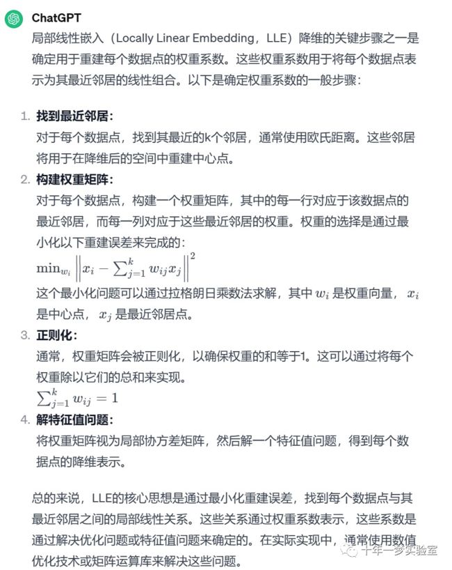
1.2.1 局部线性嵌入

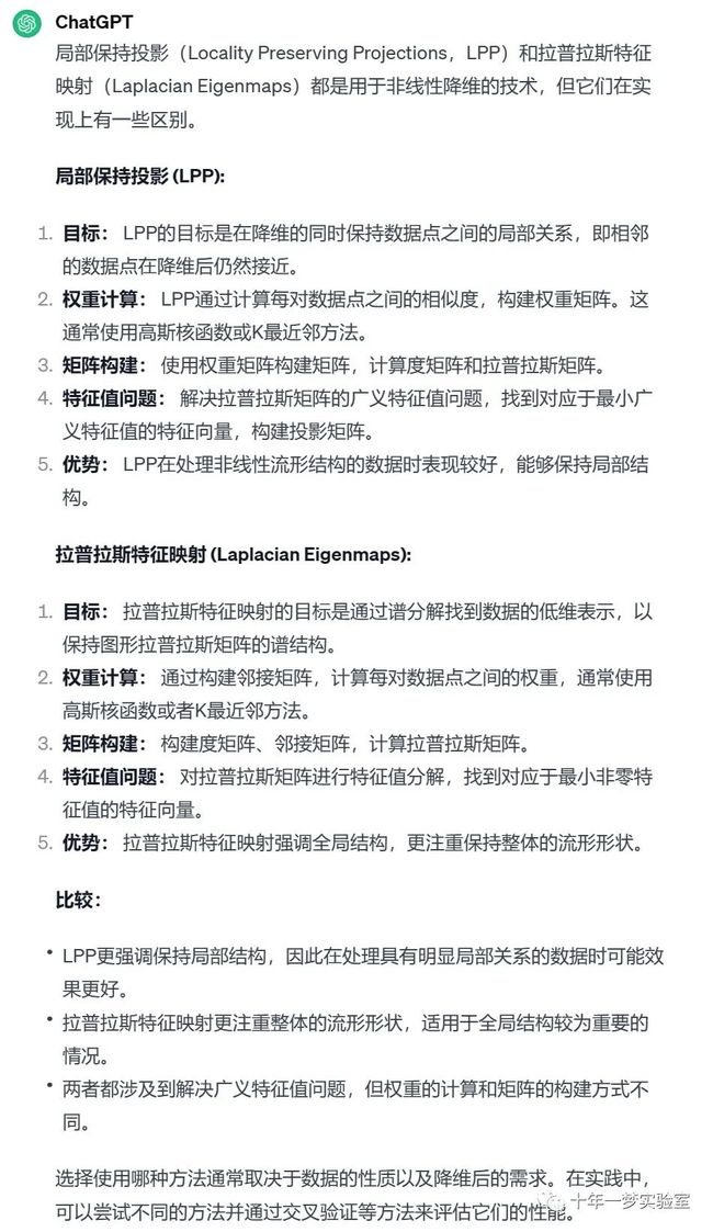
1.2.2 拉普拉斯特征映射

1.2.3 局部保持投影

1.2.4 等距映射

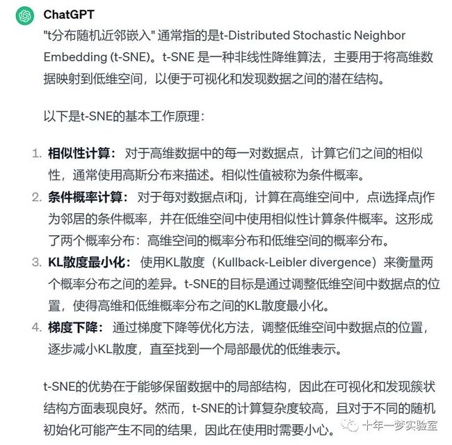
1.2.5 t分布随机近邻嵌入 

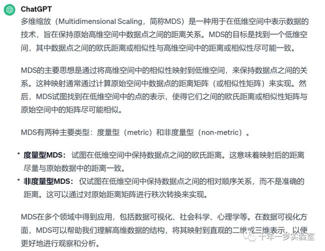
1.2.6 多维缩放

二、示例

2.1 PCA示例 iris数据集

2.2 局部线性嵌入（LLE） 瑞士卷数据降维

2.3 Swiss Roll 和 Swiss-Hole 使用 LLE 和 t-SNE 进行降维比较

# ===================================
# Swiss Roll 和 Swiss-Hole 降维比较
# ===================================


# 这个笔记旨在比较两种流行的非线性降维技术，T-分布随机邻居嵌入（t-SNE）和局部线性嵌入（LLE），在经典的 Swiss Roll 数据集上的效果。接下来，我们将探讨它们在数据中添加孔洞时的处理方式。


# %%
# Swiss Roll
# ---------------------------------------------------
#
# 首先，我们生成 Swiss Roll 数据集。


import matplotlib.pyplot as plt
from sklearn import datasets, manifold


# 生成 Swiss Roll 数据集
sr_points, sr_color = datasets.make_swiss_roll(n_samples=1500, random_state=0)


# %%
# 现在，让我们看看我们的数据：


fig = plt.figure(figsize=(8, 6))
ax = fig.add_subplot(111, projection="3d")
fig.add_axes(ax)
ax.scatter(sr_points[:, 0], sr_points[:, 1], sr_points[:, 2], c=sr_color, s=50, alpha=0.8)
ax.set_title("Swiss Roll in Ambient Space")
ax.view_init(azim=-66, elev=12)
_ = ax.text2D(0.8, 0.05, s="n_samples=1500", transform=ax.transAxes)


# %%
# 计算 LLE 和 t-SNE 的嵌入，发现 LLE 似乎能够很好地展开 Swiss Roll。另一方面，t-SNE 能够保留数据的一般结构，但较差地表示原始数据的连续性。相反，它似乎不必要地将一些点的区域聚集在一起。


# 计算 LLE 嵌入
sr_lle, sr_err = manifold.locally_linear_embedding(sr_points, n_neighbors=12, n_components=2)


# 计算 t-SNE 嵌入
sr_tsne = manifold.TSNE(n_components=2, perplexity=40, random_state=0).fit_transform(sr_points)


# 绘制嵌入结果
fig, axs = plt.subplots(figsize=(8, 8), nrows=2)
axs[0].scatter(sr_lle[:, 0], sr_lle[:, 1], c=sr_color)
axs[0].set_title("LLE Embedding of Swiss Roll")
axs[1].scatter(sr_tsne[:, 0], sr_tsne[:, 1], c=sr_color)
_ = axs[1].set_title("t-SNE Embedding of Swiss Roll")


# %%
# .. 注意::
#
#     LLE 似乎将点从 Swiss Roll 中心（紫色）拉伸出来。然而，我们观察到这只是数据生成方式的副产品。在 Swiss Roll 中心附近的点密度较大，最终影响了 LLE 在较低维度中对数据的重构。


# %%
# Swiss-Hole
# ---------------------------------------------------
#
# 现在让我们看看两种算法如何处理我们在数据中添加孔洞。首先，我们生成 Swiss-Hole 数据集并绘制它：


# 生成 Swiss-Hole 数据集
sh_points, sh_color = datasets.make_swiss_roll(n_samples=1500, hole=True, random_state=0)


fig = plt.figure(figsize=(8, 6))
ax = fig.add_subplot(111, projection="3d")
fig.add_axes(ax)
ax.scatter(sh_points[:, 0], sh_points[:, 1], sh_points[:, 2], c=sh_color, s=50, alpha=0.8)
ax.set_title("Swiss-Hole in Ambient Space")
ax.view_init(azim=-66, elev=12)
_ = ax.text2D(0.8, 0.05, s="n_samples=1500", transform=ax.transAxes)


# %%
# 计算 LLE 和 t-SNE 的嵌入，我们得到了与 Swiss Roll 类似的结果。LLE 能够很好地展开数据，甚至保留了孔洞。t-SNE 再次似乎将一些点的区域聚集在一起，但我们注意到它保留了原始数据的一般拓扑结构。


# 计算 LLE 嵌入
sh_lle, sh_err = manifold.locally_linear_embedding(sh_points, n_neighbors=12, n_components=2)


# 计算 t-SNE 嵌入
sh_tsne = manifold.TSNE(n_components=2, perplexity=40, init="random", random_state=0).fit_transform(sh_points)


# 绘制嵌入结果
fig, axs = plt.subplots(figsize=(8, 8), nrows=2)
axs[0].scatter(sh_lle[:, 0], sh_lle[:, 1], c=sh_color)
axs[0].set_title("LLE Embedding of Swiss-Hole")
axs[1].scatter(sh_tsne[:, 0], sh_tsne[:, 1], c=sh_color)
_ = axs[1].set_title("t-SNE Embedding of Swiss-Hole")


# %%
#
# 结论
# ------------------
#
# 我们注意到 t-SNE 受益于测试更多的参数组合。通过更好地调整这些参数，可能会得到更好的结果。
#
# 我们观察到，正如在 "手写数字的流形学习" 示例中所见，t-SNE 通常在真实世界的数据上表现优于 LLE。

2.4 在 S-curve 数据集上进行降维的图示，使用了各种流形学习方法

# ========================================
# 流形学习方法的比较
# ========================================


# 这是在 S-curve 数据集上进行降维的图示，使用了各种流形学习方法。


# 有关这些算法的讨论和比较，请参见 :ref:`manifold module page `。


# 对于一个类似的示例，其中这些方法应用于球体数据集，请参见 :ref:`sphx_glr_auto_examples_manifold_plot_manifold_sphere.py`


# 请注意，MDS 的目的是找到数据的低维表示（这里是2D），其中距离很好地反映原始高维空间中的距离，与其他流形学习算法不同，它不寻求在低维空间中找到各向同性的数据表示。




# 作者: Jake Vanderplas -- 


# %%
# 数据集准备
# -------------------
#
# 我们从生成 S-curve 数据集开始。


from numpy.random import RandomState
import matplotlib.pyplot as plt
from matplotlib import ticker
import warnings
warnings.filterwarnings('ignore', category=FutureWarning)
# 用于在 matplotlib < 3.2 中进行 3D 投影的未使用但必需的导入
import mpl_toolkits.mplot3d  # noqa: F401


from sklearn import manifold, datasets


rng = RandomState(0)


n_samples = 1500
S_points, S_color = datasets.make_s_curve(n_samples, random_state=rng)
plt.rcParams['font.sans-serif'] = ['SimHei']  # 用来正常显示中文标签
plt.rcParams['axes.unicode_minus'] = False  # 用来正常显示负号
# %%
# 让我们看一下原始数据。还定义一些辅助函数，我们将在后面使用。


def plot_3d(points, points_color, title):
  x, y, z = points.T


  fig, ax = plt.subplots(
    figsize=(6, 6),
    facecolor="white",
    tight_layout=True,
    subplot_kw={"projection": "3d"},
  )
  fig.suptitle(title, size=16)
  col = ax.scatter(x, y, z, c=points_color, s=50, alpha=0.8)
  ax.view_init(azim=-60, elev=9)
  ax.xaxis.set_major_locator(ticker.MultipleLocator(1))
  ax.yaxis.set_major_locator(ticker.MultipleLocator(1))
  ax.zaxis.set_major_locator(ticker.MultipleLocator(1))


  fig.colorbar(col, ax=ax, orientation="horizontal", shrink=0.6, aspect=60, pad=0.01)
  plt.show()




def plot_2d(points, points_color, title):
  fig, ax = plt.subplots(figsize=(3, 3), facecolor="white", constrained_layout=True)
  fig.suptitle(title, size=16)
  add_2d_scatter(ax, points, points_color)
  plt.show()




def add_2d_scatter(ax, points, points_color, title=None):
  x, y = points.T
  ax.scatter(x, y, c=points_color, s=50, alpha=0.8)
  ax.set_title(title)
  ax.xaxis.set_major_formatter(ticker.NullFormatter())
  ax.yaxis.set_major_formatter(ticker.NullFormatter())




plot_3d(S_points, S_color, "原始 S-curve 样本")


# %%
# 定义流形学习的算法
# -------------------------------------------
#
# 流形学习是一种非线性降维的方法。这个任务的算法基于这样一种思想，即许多数据集的维度只是人为地高。
#
# 在 :ref:`User Guide ` 中阅读更多。


n_neighbors = 12  # 用于恢复局部线性结构的邻域数量
n_components = 2  # 流形的坐标数


# %%
# 局部线性嵌入
# ^^^^^^^^^^^^^^^^^^^^^^^^^
#
# 局部线性嵌入（LLE）可以被看作是一系列局部主成分分析，这些分析在全局上进行比较以找到最佳的非线性嵌入。
# 在 :ref:`User Guide ` 中阅读更多。


params = {
  "n_neighbors": n_neighbors,
  "n_components": n_components,
  "eigen_solver": "auto",
  "random_state": rng,
}


lle_standard = manifold.LocallyLinearEmbedding(method="standard", **params)
S_standard = lle_standard.fit_transform(S_points)


lle_ltsa = manifold.LocallyLinearEmbedding(method="ltsa", **params)
S_ltsa = lle_ltsa.fit_transform(S_points)


lle_hessian = manifold.LocallyLinearEmbedding(method="hessian", **params)
S_hessian = lle_hessian.fit_transform(S_points)


lle_mod = manifold.LocallyLinearEmbedding(method="modified", modified_tol=0.8, **params)
S_mod = lle_mod.fit_transform(S_points)


# %%
fig, axs = plt.subplots(
  nrows=2, ncols=2, figsize=(7, 7), facecolor="white", constrained_layout=True
)
fig.suptitle("局部线性嵌入", size=16)


lle_methods = [
  ("标准局部线性嵌入", S_standard),
  ("局部切线空间对齐", S_ltsa),
  ("Hessian 特征图", S_hessian),
  ("修改后的局部线性嵌入", S_mod),
]
for ax, method in zip(axs.flat, lle_methods):
  name, points = method
  add_2d_scatter(ax, points, S_color, name)


plt.show()


# %%
# Isomap 嵌入
# ^^^^^^^^^^^^
#
# 通过等距映射进行的非线性降维。
# Isomap 寻求一个保持所有点之间测地距离的低维嵌入。在 :ref:`User Guide ` 中阅读更多。


isomap = manifold.Isomap(n_neighbors=n_neighbors, n_components=n_components, p=1)
S_isomap = isomap.fit_transform(S_points)


plot_2d(S_isomap, S_color, "Isomap 嵌入")


# %%
# 多维缩放
# ^^^^^^^^^
#
# 多维缩放（MDS）寻求在低维度空间中表示数据，其中距离很好地反映原始高维空间中的距离。
# 在 :ref:`User Guide ` 中阅读更多。


md_scaling = manifold.MDS(
  n_components=n_components, max_iter=50, n_init=4, random_state=rng
)
S_scaling = md_scaling.fit_transform(S_points)


plot_2d(S_scaling, S_color, "多维缩放")


# %%
# 用于非线性降维的谱嵌入
# ^^^^^^^^^^^^^^^^^^^^^^^^^^^^^^^^^^^^^^^^^^^^^^^^^^^^^^^^^
#
# 该实现使用 Laplacian Eigenmaps，通过图 Laplacian 的谱分解找到数据的低维表示。
# 在 :ref:`User Guide ` 中阅读更多。


spectral = manifold.SpectralEmbedding(
  n_components=n_components, n_neighbors=n_neighbors
)
S_spectral = spectral.fit_transform(S_points)


plot_2d(S_spectral, S_color, "谱嵌入")


# %%
# t-分布随机邻居嵌入
# ^^^^^^^^^^^^^^^^^^^^^^^^^^^^^^^^^^^^^^^^^^^
#
# 它将数据点之间的相似性转换为联合概率，并试图最小化低维嵌入和高维数据之间的 Kullback-Leibler 散度。
# t-SNE 有一个非凸的成本函数，即使用不同的初始化，我们可以得到不同的结果。在 :ref:`User Guide ` 中阅读更多。


t_sne = manifold.TSNE(
  n_components=n_components,
  learning_rate="auto",
  perplexity=30,
  n_iter=250,
  init="random",
  random_state=rng,
)
S_t_sne = t_sne.fit_transform(S_points)


plot_2d(S_t_sne, S_color, "t-分布随机邻居嵌入")

三、参考

https://zhuanlan.zhihu.com/p/37777074

https://scikit-learn.org.cn/view/107.html   流形学习

https://scikit-learn.org/stable/ 

https://www.geeksforgeeks.org/spectral-embedding/?ref=ml_lbp  光谱嵌入

https://scikit-learn.org/stable/auto_examples/manifold/plot_compare_methods.html#sphx-glr-auto-examples-manifold-plot-compare-methods-py  流形学习的方法比较

https://zhuanlan.zhihu.com/p/104655163

https://www.cnblogs.com/tgzhu/p/7389193.html

https://www.geeksforgeeks.org/locally-linear-embedding-in-machine-learning/  机器学习中的局部线性嵌入

The End