【论文笔记】RepVGG: Making VGG-style ConvNets Great Again

RepVGG: Making VGG-style ConvNets Great Again

code

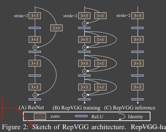
• 提出了一种在训练阶段使用多分支网络结构，但是在inference时只有3x3卷积和Relu激活函数组成的单分支网络结构。
• 网络主要用了一种结构重参数化方法a structural re-parameterization technique将训练时的多分枝融合为推理时的单分支结构。
• 因为inference时网络很像VGG结构，和使用re-parameterization方法，所以命名为RepVGG.

1. Introduction

1.1 多分支网络结构的缺点

1. 多分支的网络结构减少程序的并发性，在推理时的速度慢，降低内存利用率（比如ResNet中残差分支的add、Inception结构的concatenation操作）
2. 一些组件比如说深度可分离卷积、channel shuffle（ShuffleNets）会增加内存消耗，并且适用性不好。

1.2 RepVGG优点

很多因素影响推理速度，FLOPs的数量值不能真实反应实际的速度。

1. 网络推理时是一条单分支结构。

2. 只使用3x3卷积核ReLU激活函数。证明了kernel=3的有效性
   

3. 网络简单，没有复杂的超参数。

4. RepVGG是由RepVGGBlock堆叠的简单网络，能很好的达到速度和精度的折中。证明了该网络在分类和分割上的有效性。
   

2. Model Re-parameterization（模型重参数化）

2.1. DiracNet

通过对普通卷积进行编码得到的一条单分支网络，也是 一种 re-parameterization method。
$$W=diag(a)I+diag(b)W_{norm}$$
$W$是最终的卷积参数，$a$和$b$是一个待学习的参数，$W_{norm}$是归一化后的卷积核

另外，之前看过的ACBlock、DO-Conv 、ExpandNet也可以看作是一种模型重参数化方法，他们是把一个block看成一个卷积，去代替普通卷积，是一种component-level improvements 。而本文提出的方法对应一个扁平（plain)的卷积网络来说是很重要的。

2.2 Winograd Convolution

Winograd is a classic algorithm for accelerating 3 × 3 conv (only if the stride is 1).

3. Building RepVGG via Structural Re-param

3.1Simple is Fast, Memory-economical, Flexible

• Fast：

  • == 内存访问成本(MAC)和并发度这两个影响推理速度的关键因素没有被考虑进FLOPs，因此FLOPs其实并不能反应真实的推理速度==
  • 此外，在分组卷积中，MAC占用了很大一部分时间。另一方面，在相同的FLOPs下，一个具有高并行度的模型可能比另一个具有低并行度的模型快得多。

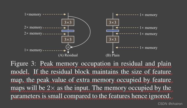
• Memory-economical

  • 多分支网络结构内存使用是无效率的，因为在add或者concatenate操作之前，每个分支的结果都需要保持，因此会导致内存占用量的峰值变高。
  • 相比之下，普通单分支网络允许在操作完成时立即释放输入到特定图层的输入所占用的内存。在设计专门的硬件时，能做更深层次的内存优化，并降低内存单元的成本，这样我们就可以将更多的计算单元集成到芯片上。

• Flexible

  • 比如残差连接，必须要相同size才能add，就需要做一些操作和限制
  • 多分枝结构限制了通道减枝（channel pruning）的运用
    

3.2 对ResNet的一段精辟解释

ResNet，它构造了一个shortcut分支来将信息流建模为$y=x+f(x)$，并使用一个残差块来学习$f$
当x和f (x)的维度不匹配时，它就变成了$y=g(x)+f(x)$，其中$g(x)$是一个由一个1×1conv实现的shortcut。对ResNets成功的一个解释是，这样的多分支体系结构使模型成为一个由许多较浅的模型[36]组成的隐式集成。

ResNet, which explicitly constructs a shortcut branch to model the information flow as y = x + f(x) and uses a residual block to learn f. When the dimensions of x and f(x) do not match, it becomes y = g(x)+f(x), where g(x)is a convolutional shortcut implemented by a 1×1 conv.

RepVGG使用了像是ResNet中的恒等连接的一个分支，并且加了一个1x1卷积分支，共三个卷积分支进行相加:$y=x+g(x)+f(x)$

3.3 Re-param for Plain Inference-time Model

训练阶段：
$$M(2)=bn(M(1)\ast W(3),\mu (3),\sigma (3),\gamma (3),\beta (3))+bn(M(1)\ast W(1),\mu (1),\sigma (1),\gamma (1),\beta (1))+bn(M(1),\mu (0),\sigma (0),\gamma (0),\beta (0)).$$
就是 $y=bn（1\ast 1Conv)+bn(3\ast 3Conv)+bn(x)$

推理阶段：

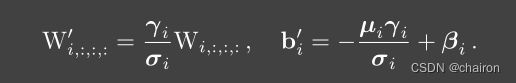
1. BN带有bias
   $$bn(M,\mu ,\sigma ,\gamma ,\beta {)}_{:,i,:,:}=(M:,i,:,:-\mu i)\frac{{\gamma }_i}{{\sigma }_i}+{\beta }_i.$$
2. 将多分支卷积进行fuse，转化为$W^{\prime }$和$b^{\prime }$作为推理时卷积的kernel和bias。其中在conv 和bn进行融合的过程中，11卷积核通过padding成为33卷积核大小，才能进行相加。同样恒等连接适用，看成是一个单位矩阵的1*1的卷积。将三个分支融合后的bias和kernel分别相加，作为推理卷积的bias和kernel。
   
   
   

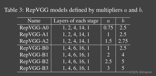
3.4. Architectural Specification

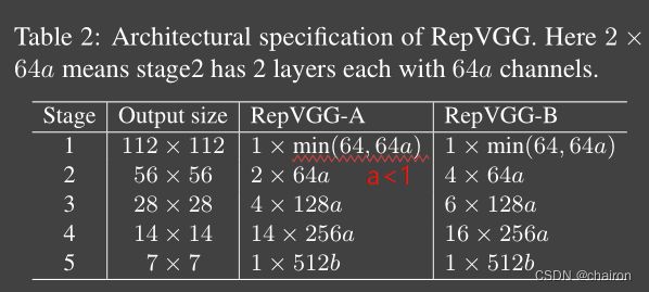
RepVGG将网络分成5个阶段

1. 第一阶段以较大的分辨率运行，很耗时，因此仅使用一层来减少延迟。
2. 最后一层有很多通道，所以只用一层来保存参数
3. RepVGG-A:1,2,4,14,1 与轻量级网络及Restnet对比； RepVGG-B:1,4,6,14,1 与高性能网络对比。
4. a>b 缩放因子，b用于最后一阶段，a用于前四阶段，第一阶段设置a<1
5. 为了进一步减少参数量和计算量，我们可能选择性的在密集部分插入3x3分组卷积

we set the number of groups $g$ the 3rd, 5th, 7th, …, 21st layer of RepVGG-A and the additional 23rd, 25th and 27th layers of RepVGG-B.
Note that the 1×1 branch shall have the same $g$ as the 3×3 conv.

4. Experiments

4.1. RepVGG for ImageNet Classification

4.2. 消融实验

• 与ACB的比较表明，REPVGG的成功不应简单地归因于每个组件过度参数化的影响，因为ACB使用了更多的参数，但性能较低。
• 准确率为76.34%，仅比ResNet-50基线高0.03%，表明repvgg的结构重参数化不是一种通用的重参数化技术，而是训练强大的普通ConvNets的关键方法。
  

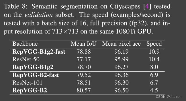
4.3. Semantic Segmentation

4.4. Limitations

RepVGG models are fast, simple and practical ConvNets designed for the maximum speed on GPU and specialized hardware, less concerning the number of parameters. They are more parameter-efficient than ResNets but may be less favored than the mobile-regime models like MobileNets[16, 30, 15] and ShuffleNets [41, 24] for low-power devices.

but may be less用的很是巧妙了，避重就轻。

5. Conclusion

We proposed RepVGG, a simple architecture with a stack of 3 × 3 conv and ReLU, which is especially suitable for GPU and specialized inference chips. With our structural re-parameterization method, it reaches over 80% top-1 accuracy on ImageNet and shows favorable speed-accuracy trade-off compared to the state-of-the-art models.

1. 提出了一个仅有3*3卷积核ReLU激活函数堆叠成的简单架构，RepVGG.尤其适合GPU和推理时间有限制的情况。
2. 在 ImageNet数据集上top-1准确率达到了80%，与最先进的模型相比，显示出良好的速度和准确率的权衡。

6. 精确度（precision）和准确率（accuracy）的区别

Precision表示被分为正例的示例中实际为正例的比例，precision=TP/（TP+FP）。即，一个二分类，类别分别命名为1和2，Precision就表示在类别1中，分对了的数量占了类别1总数量的多少；同理，也表示在类别2中，分对了的数量占类别2总数量的多少。那么这个指标越高，就表示越整齐不混乱。
而Accuracy是我们最常见的评价指标，accuracy = （TP+TN）/(P+N)，这个很容易理解，就是被分对的样本数除以所有的样本数，通常来说，正确率越高，分类器越好。我们最常说的就是这个准确率。

代码讲解

import torch.nn as nn
import numpy as np
import torch
import copy
from se_block import SEBlock
import torch.utils.checkpoint as checkpoint

def conv_bn(in_channels, out_channels, kernel_size, stride, padding, groups=1):
    result = nn.Sequential()
    result.add_module('conv', nn.Conv2d(in_channels=in_channels, out_channels=out_channels,
                                                  kernel_size=kernel_size, stride=stride, padding=padding, groups=groups, bias=False))
    result.add_module('bn', nn.BatchNorm2d(num_features=out_channels))
    return result

class RepVGGBlock(nn.Module):

    def __init__(self, in_channels, out_channels, kernel_size,
                 stride=1, padding=0, dilation=1, groups=1, padding_mode='zeros', deploy=False, use_se=False):
        super(RepVGGBlock, self).__init__()
        self.deploy = deploy
        self.groups = groups
        self.in_channels = in_channels

        assert kernel_size == 3
        assert padding == 1

        padding_11 = padding - kernel_size // 2

        self.nonlinearity = nn.ReLU()  #激活函数

        if use_se:  #是否使用SE模块
            #   Note that RepVGG-D2se uses SE before nonlinearity. But RepVGGplus models uses SE after nonlinearity.
            self.se = SEBlock(out_channels, internal_neurons=out_channels // 16)
        else:
            self.se = nn.Identity()

        if deploy: #推理阶段，只有一层卷积，没有分支：rbr_reparam
            self.rbr_reparam = nn.Conv2d(in_channels=in_channels, out_channels=out_channels, kernel_size=kernel_size, stride=stride,
                                      padding=padding, dilation=dilation, groups=groups, bias=True, padding_mode=padding_mode)

        else: #训练阶段:1. 恒等连接：rbr_identity 、2.1x1分支：rbr_1x1 3. kxk卷积分支（主分支）：rbr_dense：通常k=3
            self.rbr_identity = nn.BatchNorm2d(num_features=in_channels) if out_channels == in_channels and stride == 1 else None
            self.rbr_dense = conv_bn(in_channels=in_channels, out_channels=out_channels, kernel_size=kernel_size, stride=stride, padding=padding, groups=groups)
            self.rbr_1x1 = conv_bn(in_channels=in_channels, out_channels=out_channels, kernel_size=1, stride=stride, padding=padding_11, groups=groups)
            print('RepVGG Block, identity = ', self.rbr_identity)


    def forward(self, inputs):
        if hasattr(self, 'rbr_reparam'): #推理阶段
            return self.nonlinearity(self.se(self.rbr_reparam(inputs)))

        if self.rbr_identity is None:
            id_out = 0
        else:
            id_out = self.rbr_identity(inputs)

        #返回三个卷积分支的值
        return self.nonlinearity(self.se(self.rbr_dense(inputs) + self.rbr_1x1(inputs) + id_out))


    #   Optional. This may improve the accuracy and facilitates quantization in some cases.
    #   1.  Cancel the original weight decay on rbr_dense.conv.weight and rbr_1x1.conv.weight.
    #   2.  Use like this.
    #       loss = criterion(....)
    #       for every RepVGGBlock blk:
    #           loss += weight_decay_coefficient * 0.5 * blk.get_cust_L2()
    #       optimizer.zero_grad()
    #       loss.backward()
    def get_custom_L2(self):
        K3 = self.rbr_dense.conv.weight
        K1 = self.rbr_1x1.conv.weight
        t3 = (self.rbr_dense.bn.weight / ((self.rbr_dense.bn.running_var + self.rbr_dense.bn.eps).sqrt())).reshape(-1, 1, 1, 1).detach()
        t1 = (self.rbr_1x1.bn.weight / ((self.rbr_1x1.bn.running_var + self.rbr_1x1.bn.eps).sqrt())).reshape(-1, 1, 1, 1).detach()

        l2_loss_circle = (K3 ** 2).sum() - (K3[:, :, 1:2, 1:2] ** 2).sum()      # The L2 loss of the "circle" of weights in 3x3 kernel. Use regular L2 on them.
        eq_kernel = K3[:, :, 1:2, 1:2] * t3 + K1 * t1                           # The equivalent resultant central point of 3x3 kernel.
        l2_loss_eq_kernel = (eq_kernel ** 2 / (t3 ** 2 + t1 ** 2)).sum()        # Normalize for an L2 coefficient comparable to regular L2.
        return l2_loss_eq_kernel + l2_loss_circle



#   This func derives the equivalent kernel and bias in a DIFFERENTIABLE way.
#   You can get the equivalent kernel and bias at any time and do whatever you want,
    #   for example, apply some penalties or constraints during training, just like you do to the other models.
#   May be useful for quantization or pruning.
    def get_equivalent_kernel_bias(self):  #得到conv 和 bn 融合后的卷积：kernel、bias，并相加
        kernel3x3, bias3x3 = self._fuse_bn_tensor(self.rbr_dense)
        kernel1x1, bias1x1 = self._fuse_bn_tensor(self.rbr_1x1)
        kernelid, biasid = self._fuse_bn_tensor(self.rbr_identity)
        return kernel3x3 + self._pad_1x1_to_3x3_tensor(kernel1x1) + kernelid, bias3x3 + bias1x1 + biasid

    def _pad_1x1_to_3x3_tensor(self, kernel1x1):#将1x1卷积padding成3x3卷积
        if kernel1x1 is None:
            return 0
        else:
            return torch.nn.functional.pad(kernel1x1, [1,1,1,1])

    def _fuse_bn_tensor(self, branch): #bn 和conv 融合：inference 时 用bn对conv的权重进行归一化
        if branch is None:
            return 0, 0
        if isinstance(branch, nn.Sequential):
            kernel = branch.conv.weight
            running_mean = branch.bn.running_mean
            running_var = branch.bn.running_var
            gamma = branch.bn.weight
            beta = branch.bn.bias
            eps = branch.bn.eps
        else:
            assert isinstance(branch, nn.BatchNorm2d)
            if not hasattr(self, 'id_tensor'):
                input_dim = self.in_channels // self.groups
                kernel_value = np.zeros((self.in_channels, input_dim, 3, 3), dtype=np.float32)
                for i in range(self.in_channels):
                    kernel_value[i, i % input_dim, 1, 1] = 1
                self.id_tensor = torch.from_numpy(kernel_value).to(branch.weight.device)
            kernel = self.id_tensor
            running_mean = branch.running_mean
            running_var = branch.running_var
            gamma = branch.weight
            beta = branch.bias
            eps = branch.eps
        std = (running_var + eps).sqrt()
        t = (gamma / std).reshape(-1, 1, 1, 1)
        return kernel * t, beta - running_mean * gamma / std

    def switch_to_deploy(self): #训练阶段转换为推理阶段
        if hasattr(self, 'rbr_reparam'):
            return
        kernel, bias = self.get_equivalent_kernel_bias() #获得 1x1 、3x3、恒等连接的 bn、conv融合后的卷积
        self.rbr_reparam = nn.Conv2d(in_channels=self.rbr_dense.conv.in_channels, out_channels=self.rbr_dense.conv.out_channels,
                                     kernel_size=self.rbr_dense.conv.kernel_size, stride=self.rbr_dense.conv.stride,
                                     padding=self.rbr_dense.conv.padding, dilation=self.rbr_dense.conv.dilation, groups=self.rbr_dense.conv.groups, bias=True)
        self.rbr_reparam.weight.data = kernel
        self.rbr_reparam.bias.data = bias
        #将 融合后的卷积参数赋值给 inference时的卷积：rbr_reparam
        self.__delattr__('rbr_dense') #删掉训练阶段的三个分支rbr_dense、rbr_1x1、rbr_identity
        self.__delattr__('rbr_1x1')
        if hasattr(self, 'rbr_identity'):
            self.__delattr__('rbr_identity')
        if hasattr(self, 'id_tensor'):
            self.__delattr__('id_tensor')
        self.deploy = True

• RepVGG 就是通过构建多个RepVGGBlock组成的网络。
• inference的时候需要把模型train的多分枝模型转化为单路模型，调用switch_to_deploy()函数进行融合分支。

def repvgg_model_convert(model:torch.nn.Module, save_path=None, do_copy=True):
    if do_copy:
        model = copy.deepcopy(model)
    for module in model.modules():
        if hasattr(module, 'switch_to_deploy'): #删除bn和conv进行fuse过程中，将bn的值提取为参数时添加的变量：id_tensor
            module.switch_to_deploy()
    if save_path is not None:
        torch.save(model.state_dict(), save_path)
    return model