【优化求解】蝴蝶算法MBO matlab源码
Among them, F is the fragrance concentration, c is the perceived form, I is the stimulus intensity, and a is a power index. In our simulation of butterfly movements, the following hypothesis is proposed. First, all butterflies will emit fragrance and attract each other. Second, calculate the fitness value of each butterfly in the butterfly population, and find the butterfly with the best position. Finally, calculate the scent emitted by the butterfly. Due to the interference of the external environment, a random number p is generated to determine whether the butterfly performs a local search or a global search. The BOA algorithm is divided into three phases: the initialization phase, the iterative phase, and the final phase. The first is the initialization phase. This stage requires the creation of artificial butterflies. In this step, we first determine the size of the space, randomly place the artificial butterflies, and initialize their individual values such as aroma, health, etc. Next enter the iteration stage. Each iteration needs to decide whether to perform a global search or a local search. The global search formula is as follows, r represents a random number, x is the current position, f is the current individual aroma, and g is the most fragrant butterfly[1].\ If we choose global search, the butterfly will move towards the most fragrant butterfly in the entire butterfly population.\ ![]()
If we choose the local search, the butterfly will move a random direction and distance by itself.\ ![]()
Whether to perform a global search or a local search is determined by p. p represents a possibility. This possibility simulates the effects of wind and rain on butterflies in nature. In the code we add the variable p and compare the random number r in the equation. If r is less than p, it means that the current butterfly can move to the best butterfly position and perform a global search. Conversely, if r is greater than p, a local search is performed, and the current butterfly position is randomly moved, waiting for the next iteration. The final stage is the end phase. When we reach the maximum number of iterations or get a set error rate, we stop iteration and output the best solution.
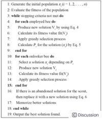
To conclude, the butterfly optimization algorithm simulates the foraging of butterflies and the way to find partners in nature. Through this algorithm, we can optimize the robot path, help save robot power and improve efficiency. It can be applied to robot scheduling in large unmanned warehouse In the system, at the same time, we can also apply the butterfly optimization algorithm to the path problem of dynamic vehicles to meet the current research boom of driverless driving.The basic concepts of the butterfly optimization algorithm were introduced earlier, and the possible improvement methods of the butterfly optimization algorithm are now introduced. The original butterfly optimization algorithm can easily fall into a local optimum, resulting in no way to obtain the global optimal solution. In addition, local and global search The ability is also limited, so people began to consider an improved butterfly optimization algorithm.In general, we have three methods to improve the global search ability of the butterfly optimization algorithm. The first is to combine the artificial bee colony algorithm. Artificial Bee Colony (ABC) is a novel swarm intelligence-based global optimization algorithm proposed by Karaboga in 2005 [4]. Its intuitive background is derived from the bee colony's honey-picking behavior. Bees perform different tasks according to their respective division of labor. Activities, and the sharing and communication of bee colony information, so as to find the optimal solution to the problem. Artificial bee colony algorithm belongs to a kind of swarm intelligence algorithm. First of all, let's first understand the basic laws of bees. Bees are a group of insects. Although the behavior of a single insect is extremely simple, a group of single individuals shows extremely complex behavior. Real bee populations can collect nectar from food sources (flowers) with high efficiency in any environment; at the same time, they can adapt to environmental changes. The minimum search model for swarm generation of swarm intelligence consists of three basic elements: food sources, hired bees, and unhired bees. Two basic behavioral models: recruiting bees for food sources and abandoning a food source. The value of the food source is determined by many factors, such as the distance from the hive, the richness of nectar, and the ease of obtaining nectar. Use a single parameter, the "yield" of the food source, to represent each of these factors. The hired bee is also called the lead bee, which corresponds to the food source collected. Leading bees store information about food sources (relative to the hive, direction, and abundance of food sources, etc.) and share this information with other bees with a certain probability. The main task of unhired bees is to find and mine food sources. There are two types of unhired bees: scout bees and followers. Scouts search for new food sources nearby; follow the bees to wait in the hive and find food sources by sharing relevant information with the lead bees. Generally, the number of detected bees is 5% -20% of the colony. Initially, the bee searches as a scout bee. The search can be determined by the prior knowledge provided by the system, or it can be completely random. After a round of investigation, if a bee finds a food source, the bee uses its own storage capacity to record location information and start collecting honey. At this point, the bee will become the "employer". After collecting honey from a food source, the bee returns to the hive to unload the honey and then has the following options. First, he can choose to abandon the food source and become a non-employed bee. Or recruit more bees for the corresponding food source and return to the food source to collect honey. Or continue to collect honey from the same food source without recruitment. For non-employed bees, you can choose to turn into a scout bee and search for food sources near the hive. The search can be determined by prior knowledge, or it can be completely random. Or be hired to follow the bee, start searching for the neighborhood of the corresponding food source and collect honey. The specific algorithm is as follows[4].
- 1
- 2
- 3
- 4
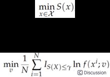
The hybrid BOA and artificial bee colony algorithm is to highlight their respective global and local search capabilities, while accelerating the convergence speed, and at the same time avoiding falling into a local optimal solution, thereby achieving global optimization.\ The second one is to add Cross-Entropy technology. Cross-Entropy (CE) was proposed by Rubinstein in 1997[2]. First let’s understand what is CE. First, we define natural information as the greater the probability of an event, the smaller the amount of information it carries. For example, the probability of Mike’s 100 points on the exam is 0.1, and his information amount is very large. 0.99, the amount of information carried is very low. Then the entropy is the expectation (E [I (x)]) of a random variable X with all the possible values of its information. Natural information can only process a single output. Entropy quantifies the total amount of uncertainty in the entire probability distribution. Entropy is actually the expected value of the amount of information. It is a measure of the uncertainty of a random variable. The greater the entropy, the greater the uncertainty of the random variable. Then Cross-Entropy is used to measure the difference between two probability distributions. The loss function is a convex function, and the global optimal solution can be found using the gradient descent method. Has a good global search ability. As long as this cross-entropy loss function is smaller, our model will be more accurate. For example, the general optimization problem is expressed by CE as:\ “Where X is a finite set of states, and S is a real-valued performance function on X.” The Kullback-Leibler divergence helps us find the best sample density[2].\ 
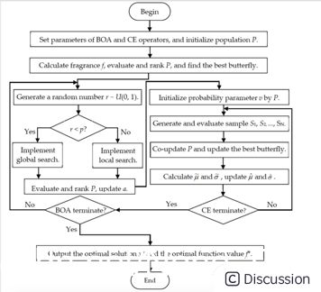
In general, cross entropy helps us to provide a faster search method and the possibility of avoiding falling into a local optimum. Then we need to combine the butterfly optimization algorithm and the cross entropy optimization algorithm. That is to say, it combines the advantages of better book search and faster convergence speed of the butterfly optimization algorithm, as well as the advantages of good CE global search and not falling into the local optimum. Synthesized BOA-CE algorithm. The specific steps are:\ The first step is to implement the butterfly optimization algorithm, following the steps introduced earlier. We need Define sensor modality c, power exponent a, and switch probability p, as well as population size and maximum number of iterations.\ In the second step, we can initialize the population P and the initial fragrance f of each individual to find the individual with the best fragrance.\ The third step generates a random number r and then compares it with switch probability p to determine whether the current individual is performing a local or global search.\ The fourth step starts the cross-entropy algorithm. We use the population P to find the probability parameter v needed in the cross-entropy.\ The fifth step is to generate and evaluate sample to find the current outstanding butterfly population.\ The sixth step is to re-evaluate with the updated excellent butterfly population to obtain the optimal (most fragrant) butterfly.\ The final step is to update the information of the optimal butterfly into the BOA algorithm, thereby forming a loop, knowing that we have reached the maximum number of iterations. The following figure clearly shows the BOA-CE algorithm process[2].\ 
Through these steps, we get the advantages of the improved butterfly optimization algorithm with better global and local search capabilities, better convergence speed, and avoiding local optimization.\ Then we use the BOA-CE algorithm to actually apply it to engineering problems, comparing the differences between before and after improvement. The first is the spring test. By setting variables, wire diameter, average coil diameter, and the number of coil turns to find the minimum weight of the spring expansion, through the following disclosure and comparison with other algorithms, we found that the BOA-CE algorithm can be found than other algorithms. Better solution[2].\ The last one is use Chaos algorithm. Chaotic system refers to a seemingly random irregular motion in a deterministic system. Its behavior is uncertain, unrepeatable, and unpredictable[3]. This is the phenomenon of chaos. Chaos comes from a non-linear dynamic system, and the dynamic system describes an arbitrary process that changes with time. This process is deterministic, similar to random, aperiodic, convergent, and extremely sensitive to initial values. Dependence. These characteristics are in line with the requirements of serial ciphers, such as logistic mapping, which is the most widely used type of nonlinear dynamical discrete chaotic mapping system. In addition, there is tent mapping, which is also a widely used class of non-linear dynamic discrete chaotic mapping systems in the fields of generation of chaotic spreading codes, construction of chaotic encryption systems, and implementation of chaotic optimization algorithms. It and the logistic map are topological conjugate maps to each other. Within the desirable range of q, the system is in a chaotic state. Then we combine chaos theory with butterfly optimization algorithm and use the dynamic characteristics of chaos theory to help the optimization algorithm search for a more comprehensive global space. First, we use chaotic mapping to generate the initial butterfly population. Previously, we used the probability p in the butterfly optimization algorithm to decide whether to perform a global search or a local search. Here we replaced p with a chaotic number. Then we also apply the spring stretching problem as an example. We can see that the chaotic butterfly optimization algorithm has a better solution than the cross-entropy butterfly optimization algorithm.\ To conclude, the butterfly optimization algorithm has the advantages of strong local search ability and fast convergence speed; however, it tends to fall into a local optimum instead of looking for a global optimum. In order to improve the global search ability of BOA, and based on co-evolution technology, we can use artificial bee colony algorithm, CE algorithm, Chaos algorithm to combine with BOA.
Reference\ [1]Arora, S., & Singh, S. (2018). Butterfly optimization algorithm: a novel approach for global optimization. Soft Computing, 23(3), 715–734. doi: 10.1007/s00500-018-3102-4
[2]Li, G., Shuang, F., Zhao, P., & Le, C. (2019). An Improved Butterfly Optimization Algorithm for Engineering Design Problems Using the Cross-Entropy Method. Symmetry, 11(8), 1049. doi: 10.3390/sym11081049
[3]Arora, S., & Singh, S. (2017). An improved butterfly optimization algorithm with chaos. Journal of Intelligent & Fuzzy Systems, 32(1), 1079–1088. doi: 10.3233/jifs-16798
[4]Arora, S., & Singh, S. (2017). An Effective Hybrid Butterfly Optimization Algorithm with Artificial Bee Colony for Numerical Optimization. International Journal of Interactive Multimedia and Artificial Intelligence, 4(4), 14. doi: 10.9781/ijimai.2017.442
4.MATLAB代码
```
% % % % % % % % % % % % % % % % % % % % % % % % % % % % % % % % % % % % %%
%% Notes:
% Different run may generate different solutions, this is determined by
% the the nature of metaheuristic algorithms.
%%
function [MinCost] = MBO(ProblemFunction, DisplayFlag, RandSeed)
% Monarch Butterfly Optimization (MBO) software for minimizing a general function
% The fixed generation is considered as termination condition.
% INPUTS: ProblemFunction is the handle of the function that returns
% the handles of the initialization, cost, and feasibility functions.
% DisplayFlag = true or false, whether or not to display and plot results.
% ProbFlag = true or false, whether or not to use probabilities to update emigration rates.
% RandSeed = random number seed
% OUTPUTS: MinCost = array of best solution, one element for each generation
% Hamming = final Hamming distance between solutions
% CAVEAT: The "ClearDups" function that is called below replaces duplicates with randomly-generated
% individuals, but it does not then recalculate the cost of the replaced individuals.
tic
if ~exist('ProblemFunction', 'var')
ProblemFunction = @Ackley;
end
if ~exist('DisplayFlag', 'var')
DisplayFlag = true;
end
if ~exist('RandSeed', 'var')
RandSeed = round(sum(100*clock));
end
[OPTIONS, MinCost, AvgCost, InitFunction, CostFunction, FeasibleFunction, ...
MaxParValue, MinParValue, Population] = Init(DisplayFlag, ProblemFunction, RandSeed);
% % % % % % % % % % % % Initial parameter setting % % % % % % % % % % % %%%%
%% Initial parameter setting
Keep = 2; % elitism parameter: how many of the best habitats to keep from one generation to the next
maxStepSize = 1.0; %Max Step size
partition = OPTIONS.partition;
numButterfly1 = ceil(partition*OPTIONS.popsize); % NP1 in paper
numButterfly2 = OPTIONS.popsize - numButterfly1; % NP2 in paper
period = 1.2; % 12 months in a year
Land1 = zeros(numButterfly1, OPTIONS.numVar);
Land2 = zeros(numButterfly2, OPTIONS.numVar);
BAR = partition; % you can change the BAR value in order to get much better performance
% % % % % % % % % % % % End of Initial parameter setting % % % % % % % % % % % %%
%%
% % % % % % % % % % % % Begin the optimization loop % % % % % % % % % %%%%
% Begin the optimization loop
for GenIndex = 1 : OPTIONS.Maxgen
% % % % % % % % % % % % Elitism Strategy % % % % % % % % % % % %%%%%
%% Save the best monarch butterflis in a temporary array.
for j = 1 : Keep
chromKeep(j,:) = Population(j).chrom;
costKeep(j) = Population(j).cost;
end
% % % % % % % % % % % % End of Elitism Strategy % % % % % % % % % % % %%%%
%%
% % % % % % % % % % % % Divide the whole population into two subpopulations % % % %%%
%% Divide the whole population into Population1 (Land1) and Population2 (Land2)
% according to their fitness.
% The monarch butterflies in Population1 are better than or equal to Population2.
% Of course, we can randomly divide the whole population into Population1 and Population2.
% We do not test the different performance between two ways.
for popindex = 1 : OPTIONS.popsize
if popindex <= numButterfly1
Population1(popindex).chrom = Population(popindex).chrom;
else
Population2(popindex-numButterfly1).chrom = Population(popindex).chrom;
end
end
% % % % % % % % % % % End of Divide the whole population into two subpopulations % % %%%
%%
% % % % % % % % % % % %% Migration operator % % % % % % % % % % % %%%%
%% Migration operator
for k1 = 1 : numButterfly1
for parnum1 = 1 : OPTIONS.numVar
r1 = rand*period;
if r1 <= partition
r2 = round(numButterfly1 * rand + 0.5);
Land1(k1,parnum1) = Population1(r2).chrom(parnum1);
else
r3 = round(numButterfly2 * rand + 0.5);
Land1(k1,parnum1) = Population2(r3).chrom(parnum1);
end
end %% for parnum1
NewPopulation1(k1).chrom = Land1(k1,:);
end %% for k1
% % % % % % % % % % % %%% End of Migration operator % % % % % % % % % % % %%%
%%
% % % % % % % % % % % % Evaluate NewPopulation1 % % % % % % % % % % % %%
%% Evaluate NewPopulation1
SavePopSize = OPTIONS.popsize;
OPTIONS.popsize = numButterfly1;
% Make sure each individual is legal.
NewPopulation1 = FeasibleFunction(OPTIONS, NewPopulation1);
% Calculate cost
NewPopulation1 = CostFunction(OPTIONS, NewPopulation1);
OPTIONS.popsize = SavePopSize;
% % % % % % % % % % % % End of Evaluate NewPopulation1 % % % % % % % % % % % %%
%%
% % % % % % % % % % % % Butterfly adjusting operator % % % % % % % % % % % %%
%% Butterfly adjusting operator
for k2 = 1 : numButterfly2
scale = maxStepSize/(GenIndex^2); %Smaller step for local walk
StepSzie = ceil(exprnd(2*OPTIONS.Maxgen,1,1));
delataX = LevyFlight(StepSzie,OPTIONS.numVar);
for parnum2 = 1:OPTIONS.numVar,
if (rand >= partition)
Land2(k2,parnum2) = Population(1).chrom(parnum2);
else
r4 = round(numButterfly2*rand + 0.5);
Land2(k2,parnum2) = Population2(r4).chrom(1);
if (rand > BAR) % Butterfly-Adjusting rate
Land2(k2,parnum2) = Land2(k2,parnum2) + scale*(delataX(parnum2)-0.5);
end
end
end %% for parnum2
NewPopulation2(k2).chrom = Land2(k2,:);
end %% for k2
% % % % % % % % % % % % End of Butterfly adjusting operator % % % % % % % % % % % %
%%
% % % % % % % % % % % % Evaluate NewPopulation2 % % % % % % % % % % % %%
%% Evaluate NewPopulation2
SavePopSize = OPTIONS.popsize;
OPTIONS.popsize = numButterfly2;
% Make sure each individual is legal.
NewPopulation2 = FeasibleFunction(OPTIONS, NewPopulation2);
% Calculate cost
NewPopulation2 = CostFunction(OPTIONS, NewPopulation2);
OPTIONS.popsize = SavePopSize;
% % % % % % % % % % % % End of Evaluate NewPopulation2 % % % % % % % % % % % %%
%%
% % % % % % % Combine two subpopulations into one and rank monarch butterflis % % % % % %
%% Combine Population1 with Population2 to generate a new Population
Population = CombinePopulation(OPTIONS, NewPopulation1, NewPopulation2);
% Sort from best to worst
Population = PopSort(Population);
% % % % % % End of Combine two subpopulations into one and rank monarch butterflis % %% % %
%%
% % % % % % % % % % % % Elitism Strategy % % % % % % % % % % % %%% %% %
%% Replace the worst with the previous generation's elites.
n = length(Population);
for k3 = 1 : Keep
Population(n-k3+1).chrom = chromKeep(k3,:);
Population(n-k3+1).cost = costKeep(k3);
end % end for k3
% % % % % % % % % % % % End of Elitism Strategy % % % % % % % % % % % %%% %% %
%%
% % % % % % % % % % Precess and output the results % % % % % % % % % % % %%%
% Sort from best to worst
Population = PopSort(Population);
% Compute the average cost
[AverageCost, nLegal] = ComputeAveCost(Population);
% Display info to screen
MinCost = [MinCost Population(1).cost];
AvgCost = [AvgCost AverageCost];
if DisplayFlag
disp(['The best and mean of Generation # ', num2str(GenIndex), ' are ',...
num2str(MinCost(end)), ' and ', num2str(AvgCost(end))]);
end
% % % % % % % % % % % End of Precess and output the results %%%%%%%%%% %% %
%%
end % end for GenIndex
Conclude1(DisplayFlag, OPTIONS, Population, nLegal, MinCost, AvgCost);
toc
% % % % % % % % % % End of Monarch Butterfly Optimization implementation %%%% %% %
%%
function [delataX] = LevyFlight(StepSize, Dim)
%Allocate matrix for solutions
delataX = zeros(1,Dim);
%Loop over each dimension
for i=1:Dim
% Cauchy distribution
fx = tan(pi * rand(1,StepSize));
delataX(i) = sum(fx);
end ```

