牛刀小试-基于LSTM的股票价格预测
前言
股票价格预测,是量化中的一种常见方式。价格预测属于一种回归任务。一般情况我们是对收盘价进行预测。价格预测的周期可以是日、周或月。
数据预处理
下面我们针对一只美股来演示如何利用LSTM对股票进行预测。
首先我们读取股票的数据:
import pandas as pd
import numpy as np
import math
import datetime as dt
from sklearn.metrics import mean_squared_error, mean_absolute_error, explained_variance_score, r2_score
from sklearn.metrics import mean_poisson_deviance, mean_gamma_deviance, accuracy_score
from sklearn.preprocessing import MinMaxScaler

import tensorflow as tf
from tensorflow.keras.models import Sequential
from tensorflow.keras.layers import Dense
from tensorflow.keras.layers import LSTM, GRU

from itertools import cycle

# ! pip install plotly
import plotly.graph_objects as go
import plotly.express as px
from plotly.subplots import make_subplots
import os
os.environ["CUDA_VISIBLE_DEVICES"] = "1"

# Import dataset
bist100 = pd.read_csv("./RELIANCE.csv")
bist100.head()
对数据的列名进行修改,并检查数据中是否有nan值,删除存在nan值的行
# Rename columns
bist100.rename(columns={"Date":"date","Open":"open","High":"high","Low":"low","Close":"close"}, inplace= True)
bist100.head()

# Checking na value
bist100.isna().any()

bist100.dropna(inplace=True)
bist100.isna().any()
将日期date转化为datetime格式,并进行排序
# convert date field from string to Date format and make it index
bist100['date'] = pd.to_datetime(bist100.date)
bist100.head()

bist100.sort_values(by='date', inplace=True)
bist100.head()
构建数据集
对收盘价数据进行缩放,缩放到0~1之间
closedf = bist100[['date','close']]
print("Shape of close dataframe:", closedf.shape)

fig = px.line(closedf, x=closedf.date, y=closedf.close,labels={'date':'Date','close':'Close Stock'})
fig.update_traces(marker_line_width=2, opacity=0.6)
fig.update_layout(title_text='Stock close price chart', plot_bgcolor='white', font_size=15, font_color='black')
fig.update_xaxes(showgrid=False)
fig.update_yaxes(showgrid=False)
fig.show()

close_stock = closedf.copy()
del closedf['date']
scaler=MinMaxScaler(feature_range=(0,1))
closedf=scaler.fit_transform(np.array(closedf).reshape(-1,1))
print(closedf.shape)
数据集进行切分,训练集占65%,测试集占35%
training_size=int(len(closedf)*0.65)
test_size=len(closedf)-training_size
train_data,test_data=closedf[0:training_size,:],closedf[training_size:len(closedf),:1]
train_data_reshape = train_data.reshape(-1)
test_data_reshape = test_data.reshape(-1)
print("train_data: ", train_data.shape)
print("test_data: ", test_data.shape)
print("train_data_reshape: ", train_data_reshape.shape)
print("test_data_reshape: ", test_data_reshape.shape)
以time_step作为一个周期,构建数据集,这里的time_step为15
# convert an array of values into a dataset matrix
def create_dataset(dataset, time_step=1):
    dataX, dataY = [], []
    for i in range(len(dataset)-time_step-1):
        a = dataset[i:(i+time_step), 0]   ###i=0, 0,1,2,3-----99   100
        dataX.append(a)
        dataY.append(dataset[i + time_step, 0])
    return np.array(dataX), np.array(dataY)

# reshape into X=t,t+1,t+2,t+3 and Y=t+4
time_step = 15
X_train, y_train = create_dataset(train_data, time_step)
X_test, y_test = create_dataset(test_data, time_step)

print("X_train: ", X_train.shape)
print("y_train: ", y_train.shape)
print("X_test: ", X_test.shape)
print("y_test", y_test.shape)
构建LSTM模型
# reshape input to be [samples, time steps, features] which is required for LSTM
X_train =X_train.reshape(X_train.shape[0],X_train.shape[1] , 1)
X_test = X_test.reshape(X_test.shape[0],X_test.shape[1] , 1)

print("X_train: ", X_train.shape)
print("X_test: ", X_test.shape)

tf.keras.backend.clear_session()
model=Sequential()
model.add(LSTM(32,return_sequences=True,input_shape=(time_step,1)))
model.add(LSTM(32,return_sequences=True))
model.add(LSTM(32))
model.add(Dense(1))
model.compile(loss='mean_squared_error',optimizer='adam')

model.summary()
模型训练
model.fit(X_train,y_train,validation_data=(X_test,y_test),epochs=100,batch_size=5,verbose=1)
模型预测
### Lets Do the prediction and check performance metrics
train_predict=model.predict(X_train)
test_predict=model.predict(X_test)

# Transform back to original form
train_predict = scaler.inverse_transform(train_predict)
test_predict = scaler.inverse_transform(test_predict)
original_ytrain = scaler.inverse_transform(y_train.reshape(-1,1))
original_ytest = scaler.inverse_transform(y_test.reshape(-1,1))
计算各种指标
# Evaluation metrices RMSE and MAE
print("Train data RMSE: ", math.sqrt(mean_squared_error(original_ytrain,train_predict)))
print("Train data MSE: ", mean_squared_error(original_ytrain,train_predict))
print("Test data MAE: ", mean_absolute_error(original_ytrain,train_predict))
print("-------------------------------------------------------------------------------------")
print("Test data RMSE: ", math.sqrt(mean_squared_error(original_ytest,test_predict)))
print("Test data MSE: ", mean_squared_error(original_ytest,test_predict))
print("Test data MAE: ", mean_absolute_error(original_ytest,test_predict))

print("Train data explained variance regression score:", explained_variance_score(original_ytrain, train_predict))
print("Test data explained variance regression score:", explained_variance_score(original_ytest, test_predict))

# R-squared (R2) is a statistical measure that represents the proportion of the variance for a dependent variable that's explained by an independent variable or variables in a regression model.

#1 = Best
#0 or < 0 = worse
print("Train data R2 score:", r2_score(original_ytrain, train_predict))
print("Test data R2 score:", r2_score(original_ytest, test_predict))

# Regression Loss Mean Gamma deviance regression loss (MGD) and Mean Poisson deviance regression loss (MPD)
print("Train data MGD: ", mean_gamma_deviance(original_ytrain, train_predict))
print("Test data MGD: ", mean_gamma_deviance(original_ytest, test_predict))
print("----------------------------------------------------------------------")
print("Train data MPD: ", mean_poisson_deviance(original_ytrain, train_predict))
print("Test data MPD: ", mean_poisson_deviance(original_ytest, test_predict))
画图对比原始收盘数据和预测收盘数据
# shift train predictions for plotting

look_back=time_step
trainPredictPlot = np.empty_like(closedf)
trainPredictPlot[:, :] = np.nan
trainPredictPlot[look_back:len(train_predict)+look_back, :] = train_predict
print("Train predicted data: ", trainPredictPlot.shape)

# shift test predictions for plotting
testPredictPlot = np.empty_like(closedf)
testPredictPlot[:, :] = np.nan
testPredictPlot[len(train_predict)+(look_back*2)+1:len(closedf)-1, :] = test_predict
print("Test predicted data: ", testPredictPlot.shape)

names = cycle(['Original close price','Train predicted close price','Test predicted close price'])


plotdf = pd.DataFrame({'date': close_stock['date'],
                       'original_close': close_stock['close'],
                      'train_predicted_close': trainPredictPlot.reshape(1,-1)[0].tolist(),
                      'test_predicted_close': testPredictPlot.reshape(1,-1)[0].tolist()})

fig = px.line(plotdf,x=plotdf['date'], y=[plotdf['original_close'],plotdf['train_predicted_close'],
                                          plotdf['test_predicted_close']],
              labels={'value':'Stock price','date': 'Date'})
fig.update_layout(title_text='Comparision between original close price vs predicted close price',
                  plot_bgcolor='white', font_size=15, font_color='black', legend_title_text='Close Price')
fig.for_each_trace(lambda t:  t.update(name = next(names)))

fig.update_xaxes(showgrid=False)
fig.update_yaxes(showgrid=False)
fig.show()
结果图:
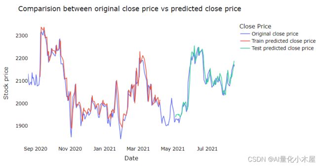
结论
从结果图可以看出,其实预测价格的趋势是挺准确的,但是如果需要预测具体的价格,确实模型很难做到,因此我们更倾向于通过模型的预测知道股票的价格在未来几天市涨或者跌,从而选择时机进行购入,而不能坚信股票价格能达到具体多少的价位。