吴恩达深度学习intuition

这里是看吴恩达课程的一些记录和联想（因为以前听过，因此不会很细致，只做个人记录）

课程链接

首先提到training set, validation set (dev set)，test set的分割问题。老师提到，最常用的划分方法传统方法是三七分（也就是training 70%，validation+test 30%，一般而言validation 20% test 10%），同时，这也是应对数据集不太大的时候的方法。也可以选择不要test set，只使用validation set做模型选择。

如果数据集很大的情况下，不采用三七分也完全可行，因为即使1%的数据量也很大，完全可以用更多的数据训练（比如98%）。

Bias-Variance trade-off

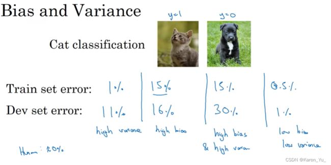
什么情况bias高？什么情况variance高？什么情况应该关注bias？什么情况应该关注variance？什么情况可以允许bias高，优先关注variance？什么情况可以允许variance高，优先关注bias？

The bias–variance trade-off implies that a model should balance underfitting and overfitting: Rich enough to express underlying structure in data and simple enough to avoid fitting spurious patterns.

简单来说，bias 和variance是用来表征是underfitting还是overfitting的。如上图，简单的判断方法就是，如果训练的效果不好，就是bias高，如果测试的效果不好，就是variance高，当然也有可能两者都低，或者两者都高。

Bias are the simplifying assumptions made by a model to make the target function easier to learn.

Generally, linear algorithms have a high bias making them fast to learn and easier to understand but generally less flexible. In turn, they have lower predictive performance on complex problems that fail to meet the simplifying assumptions of the algorithms bias.

• Low Bias: Suggests less assumptions about the form of the target function.
• High-Bias: Suggests more assumptions about the form of the target function.

Examples of low-bias machine learning algorithms include: Decision Trees, k-Nearest Neighbors and Support Vector Machines.

Examples of high-bias machine learning algorithms include: Linear Regression, Linear Discriminant Analysis and Logistic Regression.

简单来说，Bias可以描述模型的复杂情况（众所周知，模型不是越复杂越好，也不是越简单越好）。通常来说，线性算法比如y=kx+b的bias就会很高，这会导致其易于学习但不善变通。上文所举的例子中也能看出，线性的方法多导致high-bias，甚至已经加了非线性的LR也被归类到high-bias中。

Variance is the amount that the estimate of the target function will change if different training data was used.

The target function is estimated from the training data by a machine learning algorithm, so we should expect the algorithm to have some variance. Ideally, it should not change too much from one training dataset to the next, meaning that the algorithm is good at picking out the hidden underlying mapping between the inputs and the output variables.

Machine learning algorithms that have a high variance are strongly influenced by the specifics of the training data. This means that the specifics of the training have influences the number and types of parameters used to characterize the mapping function.

• Low Variance: Suggests small changes to the estimate of the target function with changes to the training dataset.
• High Variance: Suggests large changes to the estimate of the target function with changes to the training dataset.

Generally, nonlinear machine learning algorithms that have a lot of flexibility have a high variance. For example, decision trees have a high variance, that is even higher if the trees are not pruned before use.

Examples of low-variance machine learning algorithms include: Linear Regression, Linear Discriminant Analysis and Logistic Regression.

Examples of high-variance machine learning algorithms include: Decision Trees, k-Nearest Neighbors and Support Vector Machines.

variance就是使用不同的数据（这里不代表使用不同分布的数据，在课程中Ng也提到，在准备训练时，尽可能采用同分布的数据），结果也不一样，也就是我们常说的泛化能力差。一般而言，在bias上表现良好的非线性方法可能在variance上表现不佳。

In supervised learning, underfitting happens when a model unable to capture the underlying pattern of the data. These models usually have high bias and low variance. It happens when we have very less amount of data to build an accurate model or when we try to build a linear model with a nonlinear data. Also, these kind of models are very simple to capture the complex patterns in data like Linear and logistic regression.

In supervised learning, overfitting happens when our model captures the noise along with the underlying pattern in data. It happens when we train our model a lot over noisy dataset. These models have low bias and high variance. These models are very complex like Decision trees which are prone to overfitting.

我们最终的目标是期望找到一个low bias low variance的方法。但是从上面的介绍中可以看出，线性方法多具有high-bias-low-variance（underfitting）的特点，而非线性方法则恰恰相反（overfitting）。因此我们就需要提到bias-variance trade-off。（这里回答了第一个问题，什么情况bias高，什么情况variance高，当然我相信，数据的选取也很重要）

解决方案

Regime 1 (High Variance)

In the first regime, the cause of the poor performance is high variance.

Symptoms:

1. Training error is much lower than test error
2. Training error is lower than ϵ
3. Test error is above ϵ

Remedies:

• Add more training data
• Reduce model complexity -- complex models are prone to high variance
• Bagging (will be covered later in the course)

Regime 2 (High Bias)

Unlike the first regime, the second regime indicates high bias: the model being used is not robust enough to produce an accurate prediction.

Symptoms:

1. Training error is higher than ϵ

Remedies:

• Use more complex model (e.g. kernelize, use non-linear models)
• Add features
• Boosting (will be covered later in the course)

简要来说，解决bias高的方法：换模型（换成非线性方法，非线性方法虽然可能导致variance高，但你就说这个bias是不是降下来了），添加特征（也是让模型变复杂），使用boosting方法（boosting属于集成学习方法，个体学习器间存在强依赖关系、必须串行生成的序列化方法）。

解决高variance的方法：降低模型复杂度（越复杂的模型，variance越高），增加数据，使用bagging方法（属于集成学习方法，个体学习器间不存在强依赖关系、可同时生成的并行化方法(如：Bagging和“随机森林”)）

本节附录

为什么boosting可以解决high-bias？

For bagging and random forests, deep/large trees are generally employed as base learners. Large trees have high variance, but low bias. Ensembling many large trees reduces the variance.

Boosting is most effective with 'weak learners': base learners that perform slightly better than chance. Small trees generally work best, often stumps (i.e., single-split trees) are even used with boosting. Small trees have low variance, but high bias. Averaging over many trees (combined with updating the response variable after fitting each tree, which puts more weight on training observations not well predicted thus far) thus reduces the bias.

大概意思就是通过平均的方法，减少bias。在其他论述中也提到这与boosting独特的串行方法有关，因为每一轮没有得到理想结果的数据都会在下一轮训练中被重点关注。

为什么bagging可以解决high-variance？

Bootstrap aggregation, or "bagging," in machine learning decreases variance through building more advanced models of complex data sets. Specifically, the bagging approach creates subsets which are often overlapping to model the data in a more involved way.

One interesting and straightforward notion of how to apply bagging is to take a set of random samples and extract the simple mean. Then, using the same set of samples, create dozens of subsets built as decision trees to manipulate the eventual results. The second mean should show a truer picture of how those individual samples relate to each other in terms of value. The same idea can be applied to any property of any set of data points.

Since this approach consolidates discovery into more defined boundaries, it decreases variance and helps with overfitting. Think of a scatterplot with somewhat distributed data points; by using a bagging method, the engineers "shrink" the complexity and orient discovery lines to smoother parameters.

High variance models such as decision trees have a tendecy to fit closely to the noise in the dataset and can produce very unstable predictions.

Bootstrap aggregation is able to reduce the noise (variance) in the predictions by building an ensemble of models, each trained on different parts of the original dataset and aggregating the predictions produced by each model.

This is the case with not just regression models, but classification models as well.

While Bagging does also reduce bias, it has a much larger impact on the variance in the model because predictions from multiple models are being used to generate the final prediction. Noise from any single model is essentially averaged out, producing predictions that are stable and generalizable.

bagging取样的方法比较独特，每个模型都在原始数据集的不同部分进行训练，并聚合每个模型产生的预测。

Regularization

是减少variance的方法（之一，可能会增加bias）

什么是Regularization?

常见的方法就L1和L2，具体可以参考LASSO regression，Ridge regression。前者会将权重中的部分打压的很厉害，接近0。Ng提出，很多人认为采用L1 regularization可以减少权重矩阵中需要储存的数据，这样可以节约存储空间，但实际上并没有明显区别。

为什么可以减少variance？

前面提到过，线性方法容易造成high-bias-low-variance，high-bias这种就是underfitting，如果都能够造成underfitting了那肯定就不会overfitting了。无论使用哪种regularization方法，都容易把权重压到0或者近似压到0（L1或L2），就相当于数据走到这里就结束了，复杂的网络被在中途截断，那么也就不再复杂了。

同时当权重小的时候，也会带着每个node输出（下一层的输入）变小，z在较小的范围中近似于线性函数，如果每一层都是线性函数，最后组合出来的模型也就是个线性模型。因此采用这种方法本质上就是降低了非线性（复杂度），让模型变得简单，自然就不容易overfitting了。

Dropout regularization

随机失活

0.5 chance of keeping each node and 0.5 chance of removing each node.这里0.5就是keep-prop。

在课程中Ng给的例子是，先用np.random.rand创建一个随机矩阵，设定一个阈值比如np.random.rand<0.5，此时矩阵变成了一个Boolean矩阵，再将其与输入数据相乘（注意这里既然要相乘就是要大小相等了），相当于给输入的数据蒙上一层面具，值为1的地方能看到输入的数据，值为0的地方这个输入值就被失活了。

然后我们就得到了一个更简单的更小的网络。

inverted dropout

最常用的dropout方法。

Inverted dropout is a variation of the dropout technique, a popular regularization method used to prevent overfitting in neural networks. It works by randomly setting a fraction of the input units to zero at each update during training. This helps the model to learn more robust features, as it cannot rely on any single neuron too much. Inverted dropout gets its name from the modification it introduces to the standard dropout, which involves scaling the activations during training to maintain consistent expectations between the training and inference phases.

Standard dropout vs. inverted dropout

In standard dropout, a dropout mask (a binary matrix with the same shape as the input or weight matrix) is created with a certain probability, p (dropout rate), of setting elements to zero. During training, the input or weight matrix is element-wise multiplied by the dropout mask, which effectively "drops out" a fraction of neurons.

Inverted dropout modifies the standard dropout technique by scaling the remaining active neurons during training to maintain consistent expectations between the training and inference phases. This is done by dividing the result of the element-wise multiplication by the keep probability (1 - dropout rate).

其他Regularization方法

data augmentation

early stopping

Vanishing/Exploding Gradients

当训练深度网络时，有时导数会变得非常大/小（指数级别的大/小），这会为训练增加难度。

假设如上图，每个权重矩阵都是w^[l]，那么到后面1.5^L就会非常大，类似的，假设权重里的数小，最后的结果就会非常小。

Causes of Vanishing Gradient Problem

The vanishing gradient problem is often attributed to the choice of activation functions and the architecture of the neural network. Activation functions like the sigmoid or hyperbolic tangent (tanh) have gradients that are in the range of 0 to 0.25 for sigmoid and -1 to 1 for tanh. When these activation functions are used in deep networks, the gradients of the loss function with respect to the parameters can become very small, effectively preventing the weights from changing their values during training.

Another cause of the vanishing gradient problem is the initialization of weights. If the weights are initialized too small, the gradients can shrink exponentially as they are propagated back through the network, leading to vanishing gradients.

In gradient-based learning algorithms, we use gradients to learn the weights of a neural network. It works like a chain reaction as the gradients closer to the output layers are multiplied with the gradients of the layers closer to the input layers. These gradients are used to update the weights of the neural network.

If the gradients are small, the multiplication of these gradients will become so small that it will be close to zero. This results in the model being unable to learn, and its behavior becomes unstable. This problem is called the vanishing gradient problem.

解决方案

The simplest solution is to use other activation functions, such as ReLU, which doesn’t cause a small derivative.

Residual networks are another solution, as they provide residual connections straight to earlier layers. As seen in Image 2, the residual connection directly adds the value at the beginning of the block, x, to the end of the block (F(x)+x). This residual connection doesn’t go through activation functions that “squashes” the derivatives, resulting in a higher overall derivative of the block.

Finally, batch normalization layers can also resolve the issue. As stated before, the problem arises when a large input space is mapped to a small one, causing the derivatives to disappear. In Image 1, this is most clearly seen at when |x| is big. Batch normalization reduces this problem by simply normalizing the input so |x| doesn’t reach the outer edges of the sigmoid function. As seen in Image 3, it normalizes the input so that most of it falls in the green region, where the derivative isn’t too small.

使用别的激活函数，使用ResNet，批处理归一化（亦有提到在初始化时更谨慎）

Causes of Exploding Gradients

The root cause of exploding gradients can often be traced back to the network architecture and the choice of activation functions. In deep networks, when multiple layers have weights greater than 1, the gradients can grow exponentially as they propagate back through the network during training. This is exacerbated when using activation functions with outputs that are not bounded, such as the hyperbolic tangent or the sigmoid function.

Another contributing factor is the initialization of the network's weights. If the initial weights are too large, even a small gradient can be amplified through the layers, leading to very large updates during training.

An error gradient is the direction and magnitude calculated during the training of a neural network that is used to update the network weights in the right direction and by the right amount.

In deep networks or recurrent neural networks, error gradients can accumulate during an update and result in very large gradients. These in turn result in large updates to the network weights, and in turn, an unstable network. At an extreme, the values of weights can become so large as to overflow and result in NaN values.

The explosion occurs through exponential growth by repeatedly multiplying gradients through the network layers that have values larger than 1.0.

解决方案

Use Gradient Clipping

Exploding gradients can still occur in very deep Multilayer Perceptron networks with a large batch size and LSTMs with very long input sequence lengths.

If exploding gradients are still occurring, you can check for and limit the size of gradients during the training of your network.

This is called gradient clipping.

Use Weight Regularization

Another approach, if exploding gradients are still occurring, is to check the size of network weights and apply a penalty to the networks loss function for large weight values.

This is called weight regularization and often an L1 (absolute weights) or an L2 (squared weights) penalty can be used.

Use Long Short-Term Memory Networks

In recurrent neural networks, gradient exploding can occur given the inherent instability in the training of this type of network, e.g. via Backpropagation through time that essentially transforms the recurrent network into a deep multilayer Perceptron neural network.

Exploding gradients can be reduced by using the Long Short-Term Memory (LSTM) memory units and perhaps related gated-type neuron structures.

Adopting LSTM memory units is a new best practice for recurrent neural networks for sequence prediction.

类似的提出的方法，使用LSTM，regularization，梯度剪切（不给膨胀空间）

Initialization

在课程中Ng也给出了可以在一定程度上解决这些问题的方法：carefully choose the initial weights（指random initialization）

Xavier Initialization

为什么需要initialization？

在前文中也提到了，initialization对于缓解梯度的消失/爆炸有着一定的作用，但是也不能随意初始化。

If the weights are too small, then the variance of the input signal starts diminishing as it passes through each layer in the network. The input eventually drops to a really low value and can no longer be useful. 

If we use the sigmoid function as the activation function, then we know that it is approximately linear when we go close to zero. This basically means that there won’t be any non-linearity. If that’s the case, then we lose the advantages of having multiple layers.

如果把weights初始化的太小，输入随着层数的深入，variance会减小。比如用sigmoid函数作为激活函数，此函数在0的附近近似线性，在之前的内容中提到过，如果每层都近似线性，那么整个网络的模型都近似线性，线性模型属于high-bias-low-variance，虽然variance减小了，但是这个时候使用深层网络就没什么意义了，反正最后还是线性模型。（失去非线性，失去更复杂的特征，失去深层网络的作用）

If the weights are too large, then the variance of input data tends to rapidly increase with each passing layer. Eventually it becomes so large that it becomes useless. Why would it become useless? Because the sigmoid function tends to become flat for larger values, as we can see the graph above. This means that our activations will become saturated and the gradients will start approaching zero.

如果weight太大，那么非线性增加，模型更加复杂，variance增加。但是此时sigmoid函数开始趋于平坦，没有显著的变化，那么梯度也不会有显著的变化（趋近于0），此时再想gradient descend就不太能descend了。

可以参考这里的动态演示https://www.deeplearning.ai/ai-notes/initialization/index.html

Let’s illustrate the importance of initialization with an example of a model with a single hidden layer:

As you can see, the three hidden units are entirely symmetrical to the inputs.

Each hidden unit is a function of one weight coming from x1 and one from x2. If all these weights are equal, there’s no reason for the algorithm or neural network to learn that h1, h2, and h3 are different. With forward propagation, there’s no reason for the algorithm to think that even our outputs are different:

Based on this symmetry, when we’re backpropagating, all the weights are bound to be updated without distinguishing between the nodes in the net. Some optimization would still occur, so it won’t be the initial value. Still, the weights would remain useless.

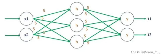
这里举了一个例子，当我们初始化时将所有的weights都初始化为一个相同的值，那么每个输入对结果的贡献都是相同的，在后续更新参数的时候可能就不会区分具体的节点（反正都一样）。

什么是Xavier initialization

Assigning the network weights before we start training seems to be a random process, right? We don’t know anything about the data, so we are not sure how to assign the weights that would work in that particular case. One good way is to assign the weights from a Gaussian distribution. Obviously this distribution would have zero mean and some finite variance. Let’s consider a linear neuron:

y = w1x1 + w2x2 + ... + wNxN + b

With each passing layer, we want the variance to remain the same. This helps us keep the signal from exploding to a high value or vanishing to zero. In other words, we need to initialize the weights in such a way that the variance remains the same for x and y. This initialization process is known as Xavier initialization. You can read the original paper here.

Xavier initialization是一种初始化方法。，采用高斯分布去分配weights。对于每一层，我们希望方差保持不变。这有助于我们防止explode/vanish。换句话说，我们需要初始化权重，使x和y的方差保持不变。高斯分布：均值为0，方差为一个有限值。

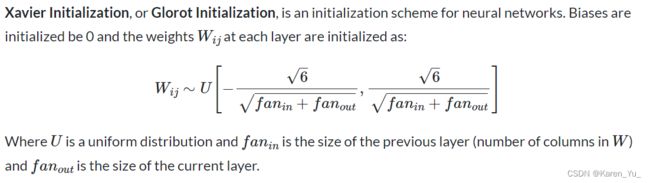
Xavier initialization怎么做

要求：

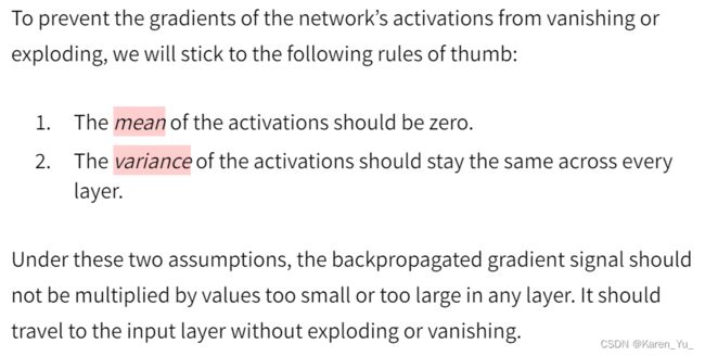
1. activations的平均值应该是零。
2. 在每一层中，activations的方差应该保持相同。

所有层的权值都是从正态分布中随机抽取的（特别说明，正态分布=高斯分布），并且要维持均值为0，方差为某特定值（该值与当前层所拥有的neuron个数相关），bias初始化为0

He Initialization

什么是He Initialization

首先pytorch支持这种初始化方法，具体可以参考https://pytorch.org/docs/stable/nn.init.html

这个函数的名字也很明确，这一方法来源于kaiming he

The he initialization method is calculated as a random number with a Gaussian probability distribution (G) with a mean of 0.0 and a standard deviation of sqrt(2/n), where n is the number of inputs to the node.

• weight = G (0.0, sqrt(2/n))

We can implement this directly in Python.

The example below assumes 10 inputs to a node, then calculates the standard deviation of the Gaussian distribution and calculates 1,000 initial weight values that could be used for the nodes in a layer or a network that uses the ReLU activation function.

After calculating the weights, the calculated standard deviation is printed as are the min, max, mean, and standard deviation of the generated weights.

The complete example is listed below.

​​​​​​​

本节附录

如何判断是vanish还是explode？

Vanishing 

• Large changes are observed in parameters of later layers, whereas parameters of earlier layers change slightly or stay unchanged
• In some cases, weights of earlier layers can become 0 as the training goes
• The model learns slowly and often times, training stops after a few iterations
• Model performance is poor

Exploding

• Contrary to the vanishing scenario, exploding gradients shows itself as unstable, large parameter changes from batch/iteration to batch/iteration
• Model weights can become NaN very quickly
• Model loss also goes to NaN

消失：后面的parameter变，前面的几乎不变；前几层就已经是0了；训练的慢或者干脆不动了；模型效果差劲

爆炸：模型的权重、损失变成NaN

————————————————————————

暂停更新，跑路去听NLP了，听完会回来继续的

参考资料

https://www.pnas.org/doi/10.1073/pnas.1903070116#:~:text=The%20bias%E2%80%93variance%20trade%2Doff%20implies%20that%20a%20model%20should,to%20avoid%20fitting%20spurious%20patterns.

https://machinelearningmastery.com/gentle-introduction-to-the-bias-variance-trade-off-in-machine-learning/

https://www.javatpoint.com/bias-and-variance-in-machine-learning

https://towardsdatascience.com/understanding-the-bias-variance-tradeoff-165e6942b229

https://www.cs.cornell.edu/courses/cs4780/2018fa/lectures/lecturenote12.html

https://stats.stackexchange.com/questions/552356/boosting-reduces-bias-when-compared-to-what-algorithm

https://www.techopedia.com/7/33193/why-does-bagging-in-machine-learning-decrease-variance

https://www.quora.com/What-is-the-reason-that-Bagging-Bootstrap-Aggregation-reduces-variance-more-than-bias-for-regression-models

https://machinelearning.wtf/terms/inverted-dropout/

https://stats.stackexchange.com/questions/207481/dropout-backpropagation-implementation

https://stats.stackexchange.com/questions/205932/dropout-scaling-the-activation-versus-inverting-the-dropout

https://deepai.org/machine-learning-glossary-and-terms/vanishing-gradient-problem

https://www.educative.io/answers/what-is-the-vanishing-gradient-problem

https://towardsdatascience.com/the-vanishing-gradient-problem-69bf08b15484

https://deepai.org/machine-learning-glossary-and-terms/exploding-gradient-problem

https://machinelearningmastery.com/exploding-gradients-in-neural-networks/

https://neptune.ai/blog/vanishing-and-exploding-gradients-debugging-monitoring-fixing

https://prateekvjoshi.com/2016/03/29/understanding-xavier-initialization-in-deep-neural-networks/

https://365datascience.com/tutorials/machine-learning-tutorials/what-is-xavier-initialization/

https://paperswithcode.com/method/xavier-initialization#:~:text=Xavier%20Initialization%2C%20or%20Glorot%20Initialization,a%20n%20o%20u%20t%20%5D

https://www.deeplearning.ai/ai-notes/initialization/index.html

https://paperswithcode.com/method/he-initialization

Weight Initialization for Deep Learning Neural Networks - MachineLearningMastery.com