For a while (at least several months since many people began to implement it with Python and/or Theano, PyLearn2 or something like that), nearly I’ve given up practicing Deep Learning with R and I’ve felt I was left alone much further away from advanced technology…
But now we have a great masterpiece: {h2o}, an implementation of H2O framework in R. I believe {h2o} is the easiest way of applying Deep Learning technique to our own datasets because we don’t have to even write any code scripts but only to specify some of its parameters. That is, using {h2o} we are free from complicated codes; we can only focus on its underlying essences and theories.
With using {h2o} on R, in principle we can implement “Deep Belief Net”, that is the original version of Deep Learning*1. I know it’s already not the state-of-the-art style of Deep Learning, but it must be helpful for understanding how Deep Learning works on actual datasets. Please remember a previous post of this blog that argues about how decision boundaries tell us how each classifier works in terms of overfitting or generalization, if you already read this blog. :)
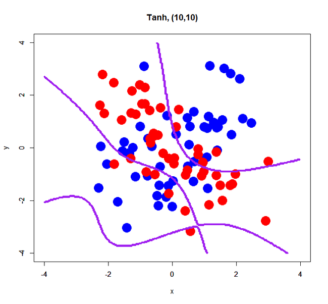
It’s much simple how to tell which overfits or well gets generalized with the given dataset generated by 4 sets of fixed 2D normal distribution. My points are: 1) if decision boundaries look well smoothed, they’re well generalized, 2) if they look too complicated, they’re overfitting, because underlying true distributions can be clearly divided into 4 quadrants with 2 perpendicular axes.
OK, let’s run the same trial with Deep Learning of {h2o} on R in order to see how DL works on the given dataset.
Datasets
Please get 3 datasets from my repository on GitHub:
simple XOR pattern, complex XOR pattern, and a grid dataset.
Github Repo for the current post. Of course, feel free to clone it; but any pull request will be rejected because this repository is not for software development. :P)
Getting started with {h2o} on R
First of all, H2O itself requires Java Virtual Machine environment. Prior to installing {h2o}, you have to install the latest version of Java SE SDK*2.
Next, {h2o} is not distributed via CRAN but available on GitHub. In order to install it, you have to add some arguments to run install.packages function.
> install.packages("h2o", repos=(c("http://s3.amazonaws.com/h2o-release/h2o/master/1542/R", getOption("repos")))) > library("h2o", lib.loc="C:/Program Files/R/R-3.0.2/library") ---------------------------------------------------------------------- Your next step is to start H2O and get a connection object (named 'localH2O', for example): > localH2O = h2o.init() For H2O package documentation, ask for help: > ??h2o After starting H2O, you can use the Web UI at http://localhost:54321 For more information visit http://docs.0xdata.com ---------------------------------------------------------------------- At any rate, now you can run {h2o} in R.
How {h2o} works on R
Once {h2o} package loaded, first you have to boot an H2O instance on Java VM. In the case below “nthreads” argument was set to -1, that means all CPU cores must be used for the H2O instance. If you want spare any cores, specify the number of cores you want to use for H2O, e.g. 7 or 6.
> localH2O <- h2o.init(ip = "localhost", port = 54321, startH2O = TRUE,
 nthreads=-1)

H2O is not running yet, starting it now...

Note:  In case of errors look at the following log files:
    C:\Users\XXX\AppData\Local\Temp\RtmpghjvGo/h2o_XXX_win_started_from_r.out C:\Users\XXX\AppData\Local\Temp\RtmpghjvGo/h2o_XXX_win_started_from_r.err java version "1.7.0_67" Java(TM) SE Runtime Environment (build 1.7.0_67-b01) Java HotSpot(TM) 64-Bit Server VM (build 24.65-b04, mixed mode) Successfully connected to http://localhost:54321 R is connected to H2O cluster: H2O cluster uptime: 1 seconds 506 milliseconds H2O cluster version: 2.7.0.1542 H2O cluster name: H2O_started_from_R H2O cluster total nodes: 1 H2O cluster total memory: 7.10 GB H2O cluster total cores: 8 H2O cluster allowed cores: 8 H2O cluster healthy: TRUE
Now you can run all functions of {h2o} package. Then load the simple XOR pattern and the grid dataset.
> cfData <- h2o.importFile(localH2O, path = "xor_simple.txt") > pgData<-h2o.importFile(localH2O,path="pgrid.txt")
We’re ready to draw various decision boundaries using {h2o} package, in particular with Deep Learning. Let’s go to the next step.
Prior to trying Deep Learning, see the previous result
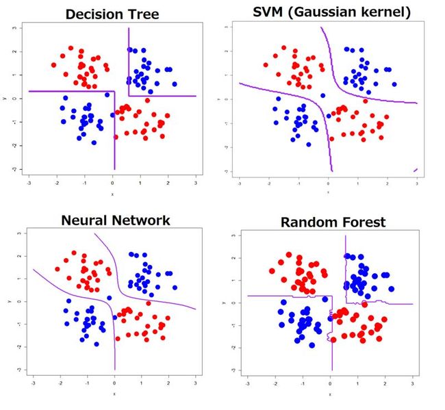
To compare a result of Deep Learning with ones of the other classifiers, please see the previous result. In the ones below, I ran decision tree, SVM with some sets of parameters, neural network (with only a hidden layer), and random forest.
Linearly inseparable and simple XOR pattern
As clearly seen, all of the classifiers showed decision boundaries well reflecting its true distribution.
Linearly inseparable and complex XOR pattern
In contrast to the simple XOR pattern, the result showed a wide variety of decision boundaries. Decision tree, neural network and random forest estimated much more complicated boundaries than the true boundaries, although SVM with well generalized by specific parameters gave natural and well smoothed boundaries (but classification accuracy was not good).
OK, let’s run h2o.deeplearning function to estimate decision boundaries using Deep Learning.
Our primary interest here is what kind of set of tuning parameters shows what kind of decision boundaries. In h2o.deeplearning function, we can tune parameters (arguments) below:
- activation: Tanh, Rectifier and Maxout. We can also add “WithDropout” to implement the dropout procedure.
- hidden: details of hidden layers, by vector. c(3,2) means 1st hidden layer with 3 units and 2nd one with 2 units. rep(3,3) means 3 consecutive hidden layers with 3 units.
- epochs: the number of iteration. Of course larger epochs, more trained output you can get.
- autoencoder: logical value that determines whether autoencoder is used or not. Here we ignore it because the sample size is too small.
- hidden_dropout_ratio: dropout ratio of hidden layers by vector. Even if you want to implement the dropout procedure, we recommend to specify only 0.5 according to Baldi (NIPS, 2013).
For simplification, in this post I only tune “activation” and “hidden”. In particular about “hidden”, the number of hidden layers are fixed to 2 or 3 and the number of units are fixed to 5 or 10. Anyway we can run it as below.
> res.dl<-h2o.deeplearning(x=1:2,y=3,data=xorsData,classification=T, activation="Tanh",hidden=c(10,10),epochs=10) > prd.dl<-h2o.predict(res.dl,newdata=pgData) > prd.dl.df<-as.data.frame(prd.dl) > xors <- read.table("xor_simple.txt", header=T) > plot(xors[,-3], pch=19, col=c(rep('blue',50), rep('red',50)), cex=3, xlim=c(-4,4), ylim=c(-4,4), main="Tanh, (10,10)") > par(new=T) > contour(px, py, array(prd.dl.df[,1], dim=c(length(px), length(py))), xlim=c(-4,4), ylim=c(-4,4), col="purple", lwd=3,drawlabels=F)
A script above is just an example; please rewrite or adjust it to your environment.
simple XOR pattern with 2 hidden layers
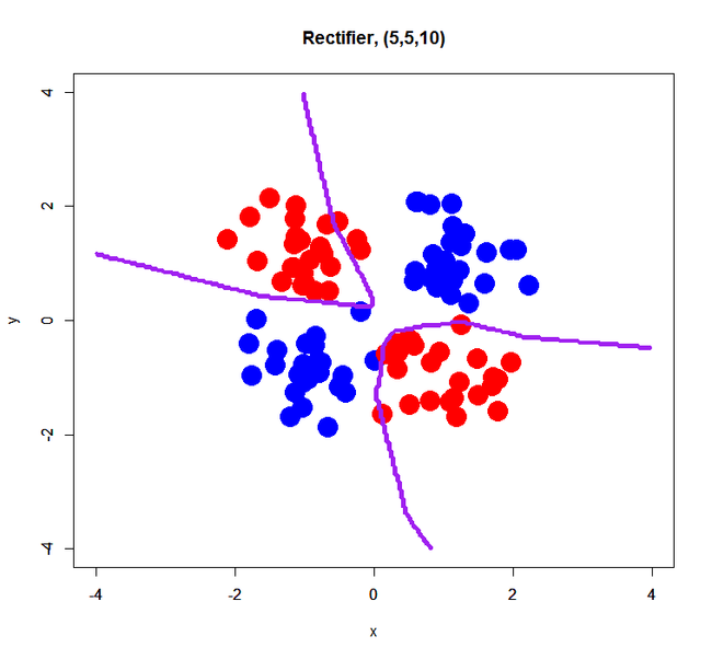
Rectifier
Maxout
Maxout failed to estimate a classification model correctly… perhaps it was caused by too small sample size (only 100) or too small dimension (just 2D). On the other hand, Tanh and Rectifier showed fairly good decision boundaries.
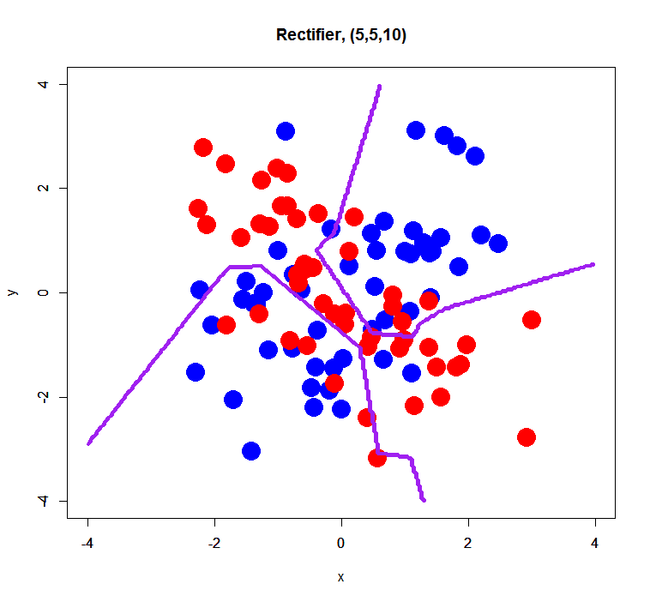
complex XOR pattern with 2 hidden layers
simple XOR pattern with 3 hidden layers
This is just a trial for evaluating an effect of the number of hidden layers. Prior to this trial, I think its number may affect a bit results of classification… so, how was it?
Rectifier


