XGBoost建模调参-保险赔偿预测模型

内容简介

保险赔偿预测模型的建立流程，主要分为了解数据和建模两大部分。第二部分建模过车着重学习如何用XGboost进行建模和调参。

• 基本建模流程：
  1）读取数据；2）特征理解；3）数据清洗、预处理；4）建立模型；5）模型评估。

1.了解数据

## 导入相关模块和数据
import pandas as pd
import numpy as np
import matplotlib.pyplot as plt
from sklearn.linear_model import LogisticRegression
from sklearn.ensemble import RandomForestClassifier
from sklearn.metrics import roc_auc_score as AUC
from sklearn.metrics import mean_absolute_error
from sklearn.decomposition import PCA
from sklearn.preprocessing import LabelEncoder, LabelBinarizer
from sklearn.model_selection import cross_val_score #Update成 mdel_selection

from scipy import stats
import seaborn as sns
from copy import deepcopy

%matplotlib inline

# This may raise an exception in earlier versions of Jupyter
%config InlineBackend.figure_format = 'retina'

#导入数据
train = pd.read_csv('train.csv')
test = pd.read_csv('test.csv')

1）了解数据基本特征

常用方法：
1）train.shape 查看数据形状，有几行几列
2）print(train.columns) 查看每列标题: 数据量少时；
print(train.columns[:20])数据量多时，提取部分标题，比如前20个：
2）train.describe()描述性分析
3）train.info()查看特征属性
4）pd.isnull(train).values.any()查看缺失值，若返回为False则无缺失值。

结果输出：
结论：

• 188k训练实例，132列;
• 有116个种类属性（如它们的名字所示）和14个连续（数字）属性，还有ID和赔偿。总计为132列。
• 所有的连续值已被缩放到[0,1]区间，均值基本为0.5
• 无缺失值
• 数据已经被预处理了

2)清洗和预处理（略）

• 数据已经预处理过，没有缺失值，可以直接用

3)确认特征属性

之前已经用了 train.info()得出结果 float64(15), int64(1), object(116)，意味着 15个浮点型、1个int,116个obj ， 接下来的步骤是进一步确认核对。

cat_features = list(train.select_dtypes(include=['object']).columns)
print("Categorical: {} features".format(len(cat_features)))

cont_features = [cont for cont in list(train.select_dtypes(
                 include=['float64', 'int64']).columns) if cont not in ['loss', 'id']] #排除掉loss和ID
print("Continuous: {} features".format(len(cont_features)))

id_col = list(train.select_dtypes(include=['int64']).columns)
print ("A column of int64: {}".format(id_col))

结果输出：

3.1)类别值 caterogical features

• 类别值中属性的个数：统计每个类别中，有多少个属性。

#统计类别属性值：
cat_uniques = []
for cat in cat_features:
    cat_uniques.append(len(train[cat].unique()))
    
#新建一个表格，一列写特征名字，另一列写该特征的属性个数
d = {'cat_name': cat_features, 'unique_values': cat_uniques}
uniq_values_in_categories = pd.DataFrame(data=d)

#看前5个类别结果
uniq_values_in_categories.head()

结果输出：

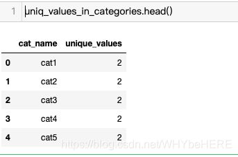
结论： 看表格，cat1到cat5都只有两个类别，比如性别就是只有男或女两个类别。

#画图，结果可视化
fig, (ax1, ax2) = plt.subplots(1,2)
fig.set_size_inches(16,5)
ax1.hist(uniq_values_in_categories.unique_values, bins=50)
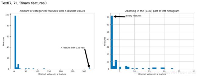
ax1.set_title('Amount of categorical features with X distinct values')
ax1.set_xlabel('Distinct values in a feature')
ax1.set_ylabel('Features')
ax1.annotate('A feature with 326 vals', xy=(322, 2), xytext=(200, 38), arrowprops=dict(facecolor='black'))

ax2.set_xlim(2,30)
ax2.set_title('Zooming in the [0,30] part of left histogram')
ax2.set_xlabel('Distinct values in a feature')
ax2.set_ylabel('Features')
ax2.grid(True)
ax2.hist(uniq_values_in_categories[uniq_values_in_categories.unique_values <= 30].unique_values, bins=30)
ax2.annotate('Binary features', xy=(3, 71), xytext=(7, 71), arrowprops=dict(facecolor='black'))

结果输出：

结论：

• X轴表示每个特征里有几种类别（值），Y表示同样类别数量的特征有几个。
• 左图表示了全部结果，右图将左边的前0-30放大。
• 结论：部分的分类特征（72/116）是二值的，绝大多数特征（88/116）有四个值，其中有一个具有326个值的特征（可能是日期）。

4)Loss（目标值Y）

#画图看ID和Loss value的关系
plt.figure(figsize=(16,8))
plt.plot(train['id'], train['loss'])
plt.title('Loss values per id')
plt.xlabel('id')
plt.ylabel('loss')
plt.legend()
plt.show()

结果输出：

结论：

• X为ID Y为Loss。由图可见，大部分Loss损失值40000一下，但是有几个显著的峰值表示严重事故。这样的数据分布会让的回归表现不佳。

偏度（skewness）概念

也称为偏态、偏态系数，是统计数据分布偏斜方向和程度的度量，是统计数据分布非对称程度的数字特征。
正态分布的偏度为0，两侧尾部长度对称。若以bs表示偏度。

• bs<0称分布具有负偏离，也称左偏态，此时数据位于均值左边的比位于右边的少，直观表现为左边的尾部相对于与右边的尾部要长，因为有少数变量值很小，使曲线左侧尾部拖得很长；

• bs>0称分布具有正偏离，也称右偏态，此时数据位于均值右边的比位于左边的少，直观表现为右边的尾部相对于与左边的尾部要长，因为有少数变量值很大，使曲线右侧尾部拖得很长；

• bs接近0则可认为分布是对称的。 若知道分布有可能在偏度上偏离正态分布时，可用偏离来检验分布的正态性。右偏时一般算术平均数>中位数>众数，左偏时相反，即众数>中位数>平均数。正态分布三者相等。
  

• 用stats.mstats.skew(train['loss']).data计算倾斜程度，如果>1, 利用对数np.log变换降低偏度

#计算偏度
stats.mstats.skew(train['loss']).data
#对数转换
stats.mstats.skew(np.log(train['loss'])).data
#画图表示
fig, (ax1, ax2) = plt.subplots(1,2)
fig.set_size_inches(16,5)
ax1.hist(train['loss'], bins=50)
ax1.set_title('Train Loss target histogram')
ax1.grid(True)
# 画直方图
ax2.hist(np.log(train['loss']), bins=50, color='g')
ax2.set_title('Train Log Loss target histogram')
ax2.grid(True)
plt.show()

输出结果：

• 经过对数转化后，偏度从3.79降低到0.092，从正/右偏态变成了一个相对标准的正态分布。

4)连续值特征Continuous features

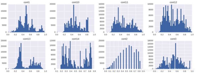
画直方图，分析每个连续值特征的分布

train[cont_features].hist(bins=50, figsize=(16,12))

部分结果展示：

相关系数(Correlation coefficient)概念

研究变量之间线性相关程度的量，一般用字母 r 表示。
相关系数的值介于–1与+1之间，即–1≤r≤+1。其性质如下：

• 当r>0时，表示两变量正相关，r<0时，两变量为负相关。
• 当|r|=1时，表示两变量为完全线性相关，即为函数关系。
• 当r=0时，表示两变量间无线性相关关系。
• 当0<|r|<1时，表示两变量存在一定程度的线性相关。且|r|越接近1，两变量间线性关系越密切；|r|越接近于0，表示两变量的线性相关越弱。
• 一般可按三级划分：|r|<0.4为低度线性相关；0.4≤|r|<0.7为显著性相关；0.7≤|r|<1为高度线性相关。

多重共线性（Multicollinearity）概念

共线性，即同线性或同线型。统计学中，共线性即多重共线性。
多重共线性（Multicollinearity）是指线性回归模型中的解释变量之间由于存在精确相关关系或高度相关关系而使模型估计失真或难以估计准确。
参考经验：如何使用简单相关系数来判断是否存在多重共线性

特征相关性，有共线性的特征不利于建模，需要剔除；利用热力图找出特征

plt.subplots(figsize=(16,9))
correlation_mat = train[cont_features].corr()
sns.heatmap(correlation_mat, annot=True)

部分结果展示： 几个特征之间有很高的相关性。

2. XGBoost建模

经过第一部分，已经基本了解数据的情况，第二部分我们直接利用已知的信息，重新另起文件，开始进入建模过程。

1）导入工具包

import xgboost as xgb
import pandas as pd
import numpy as np
import pickle
import sys
import matplotlib.pyplot as plt
from sklearn.metrics import mean_absolute_error, make_scorer
from sklearn.preprocessing import StandardScaler
from sklearn.model_selection import GridSearchCV #原本是from sklearn.grid_search import GridSearchCV
from scipy.sparse import csr_matrix, hstack
from sklearn.model_selection import KFold, train_test_split # 原from sklearn.cross_validation import KFold, train_test_split
from xgboost import XGBRegressor

import warnings
warnings.filterwarnings('ignore')

%matplotlib inline

# This may raise an exception in earlier versions of Jupyter
%config InlineBackend.figure_format = 'retina'

2）数据预处理

#重新导入数据
train = pd.read_csv('train.csv')

#做对数转换
train['log_loss'] = np.log(train['loss'])

#将数据分成连续和离散特征
features = [x for x in train.columns if x not in ['id','loss', 'log_loss']] #取出除了ID、loss和log_loss的特征

#选择object
cat_features = [x for x in train.select_dtypes(
        include=['object']).columns if x not in ['id','loss', 'log_loss']]

#用‘exclude’，选择非object
num_features = [x for x in train.select_dtypes(
        exclude=['object']).columns if x not in ['id','loss', 'log_loss']]
#打印看下结果
print ("Categorical features:", len(cat_features))
print ("Numerical features:", len(num_features))

结果显示：
Categorical features: 116
Numerical features: 14

3）数据集切分

#数据集切分
ntrain = train.shape[0]

train_x = train[features]
train_y = train['log_loss']

#将类别值转化为连续值特征。
for c in range(len(cat_features)):
    train_x[cat_features[c]] = train_x[cat_features[c]].astype('category').cat.codes
    
print ("Xtrain:", train_x.shape)
print ("ytrain:", train_y.shape)

结果显示：
Xtrain: (188318, 130)
ytrain: (188318,)

4）建立模型：

4.1）建立一个基本模型（Simple XGBoost Model）

训练一个基本的xgboost模型，然后进行参数调节通过交叉验证来观察结果的变换，使用平均绝对误差来衡量

• 平均绝对误差：
  mean_absolute_error(np.exp(y), np.exp(yhat))。用e的y次幂扩大差异性 ， 把损失值放大

#评估衡量方法：平均绝对误差
def xg_eval_mae(yhat, dtrain):
    y = dtrain.get_label()
    return 'mae', mean_absolute_error(np.exp(y), np.exp(yhat))

• xgboost 自定义了一个数据矩阵类 DMatrix，会在训练开始时进行一遍预处理，从而提高之后每次迭代的效率；

##把X和y传入DMatrix中进行处理
dtrain = xgb.DMatrix(train_x, train['log_loss'])

#按照经验值选一个参数
xgb_params = {
    'seed': 0,
    'eta': 0.1,
    'colsample_bytree': 0.5,
    'silent': 1,
    'subsample': 0.5,
    'objective': 'reg:linear',
    'max_depth': 5,
    'min_child_weight': 3
}

各项参数意义：

• ‘booster’:‘gbtree’,
• ‘objective’: ‘multi:softmax’, 多分类的问题
• ‘num_class’:10, 类别数，与 multisoftmax 并用
• ‘gamma’:损失下降多少才进行分裂
• ‘max_depth’:12, 构建树的深度，越大越容易过拟合
• ‘lambda’:2, 控制模型复杂度的权重值的L2正则化项参数，参数越大，模型越不容易过拟合。
• ‘subsample’:0.7, 随机采样训练样本
• ‘colsample_bytree’:0.7, 生成树时进行的列采样
• ‘min_child_weight’:3, 孩子节点中最小的样本权重和。如果一个叶子节点的样本权重和小于min_child_weight则拆分过程结束
• ‘silent’:0 ,设置成1则没有运行信息输出，最好是设置为0.
• ‘eta’: 0.007, 如同学习率
• ‘seed’:1000,
• ‘nthread’:7, cpu 线程数

#使用交叉验证 xgb.cv
%%time
bst_cv1 = xgb.cv(xgb_params, dtrain, num_boost_round=50, nfold=3, seed=0, feval=xg_eval_mae, maximize=False, early_stopping_rounds=10)

#打印结果
print ('CV score:', bst_cv1.iloc[-1,:]['test-mae-mean'])
#可视化结果
plt.figure()
bst_cv1[['train-mae-mean', 'test-mae-mean']].plot()

各项参数定义：
xgb_params：设定的参数
dtrain：X、Y经过xgb.DMatrix 处理组成的矩阵
num_boost_round
nfold：做几折 seed随机种子
feval 测评方法 maximize=False,
early_stopping_rounds=10

结果显示：
CV score: 1220.054769
CPU times: user 4min 54s, sys: 6.36 s, total: 5min
Wall time: 1min 39

我们的第一个基准结果：MAE＝1218.9。从图可以看出，随着迭代进行，损失值在下降， 没有发生过拟合，树模型个数为50个。

4.2）第二个模型（100棵树）

%%time
#建立100个树模型
bst_cv2 = xgb.cv(xgb_params, dtrain, num_boost_round=100, 
                nfold=3, seed=0, feval=xg_eval_mae, maximize=False, 
                early_stopping_rounds=10)

print ('CV score:', bst_cv2.iloc[-1,:]['test-mae-mean'])

#画图
fig, (ax1, ax2) = plt.subplots(1,2)
fig.set_size_inches(16,4)

ax1.set_title('100 rounds of training')
ax1.set_xlabel('Rounds')
ax1.set_ylabel('Loss')
ax1.grid(True)
ax1.plot(bst_cv2[['train-mae-mean', 'test-mae-mean']])
ax1.legend(['Training Loss', 'Test Loss'])

ax2.set_title('60 last rounds of training')
ax2.set_xlabel('Rounds')
ax2.set_ylabel('Loss')
ax2.grid(True)
ax2.plot(bst_cv2.iloc[40:][['train-mae-mean', 'test-mae-mean']])
ax2.legend(['Training Loss', 'Test Loss'])

结果输出：
CV score: 1171.2875163333333
CPU times: user 9min 44s, sys: 8.01 s, total: 9min 52s
Wall time: 3min 11s

• MAE = 1171.77 比第一次的要好 (1218.9).
• 从图中看， 在40-100区域，Test loss>Train Loss, 模型在训练集（Train）中表现很好，但是对测试集（Test）拟合不好，表明模型稍微有些过拟合。

5）参数调节

上面我们先看了树的数量对模型的影响，接下来看下其他的参数。

• Step 1: 选择一组初始参数
• Step 2: 改变 max_depth 和 min_child_weight.控制着树模型的复杂程度和深度。
• Step 3: 调节 gamma 降低模型过拟合风险. 控制分裂任务：一次分裂至少要达到什么标准才能去做？
• Step 4: 调节 subsample 和 colsample_bytree 改变数据采样策略. 按行还是按列？
• Step 5: 调节学习率 eta.

先指定xgboost类。

#类
class XGBoostRegressor(object):
    #一些不会变的参数我们把它固定下来
    def __init__(self, **kwargs):
        self.params = kwargs
        if 'num_boost_round' in self.params:
            self.num_boost_round = self.params['num_boost_round']
        self.params.update({'silent': 1, 'objective': 'reg:linear', 'seed': 0})
        
    #训练模型   
    def fit(self, x_train, y_train):
        dtrain = xgb.DMatrix(x_train, y_train) #把X和Y做成dmatrix格式
        self.bst = xgb.train(params=self.params, dtrain=dtrain, num_boost_round=self.num_boost_round, feval=xg_eval_mae, maximize=False) #用当前参数训练数据集
        
    #预测结果
    def predict(self, x_pred):
        dpred = xgb.DMatrix(x_pred)
        return self.bst.predict(dpred) 
    
    #交叉验证
    def kfold(self, x_train, y_train, nfold=5):
        dtrain = xgb.DMatrix(x_train, y_train)
        cv_rounds = xgb.cv(params=self.params, dtrain=dtrain, num_boost_round=self.num_boost_round,
                           nfold=nfold, feval=xg_eval_mae, maximize=False, early_stopping_rounds=10)
        return cv_rounds.iloc[-1,:]
   
    #画个图
    def plot_feature_importances(self):
        feat_imp = pd.Series(self.bst.get_fscore()).sort_values(ascending=False)
        feat_imp.plot(title='Feature Importances')
        plt.ylabel('Feature Importance Score')
        
    def get_params(self, deep=True):
        return self.params
 
    def set_params(self, **params):
        self.params.update(params)
        return self

#指定衡量标准
def mae_score(y_true, y_pred):
    return mean_absolute_error(np.exp(y_true), np.exp(y_pred))

mae_scorer = make_scorer(mae_score, greater_is_better=False)

Step 1: 基准模型（上面已经做过）

bst = XGBoostRegressor(eta=0.1,
colsample_bytree=0.5, subsample=0.5, max_depth=5, min_child_weight=3, num_boost_round=50)

#交叉验证                       
bst.kfold(train_x, train_y, nfold=5)

结果显示：
test-mae-mean 1219.014551
test-mae-std 8.931061
train-mae-mean 1210.682813
train-mae-std 2.798608
Name: 49, dtype: float64

开始调参

Step 2: 树的深度与节点权重

这些参数对xgboost性能影响最大，因此，他们应该调整第一。我们简要地概述它们：

• max_depth: 树的最大深度。增加这个值会使模型更加复杂，也容易出现过拟合，深度3-10是合理的。这里取了4-9
• min_child_weight: 正则化参数. 如果树分区中的实例权重小于定义的总和，则停止树构建过程。这里取1，3，6

#设置需要调整的参数
xgb_param_grid = {'max_depth': list(range(4,9)), 'min_child_weight': list((1,3,6))}
xgb_param_grid['max_depth'] 

结果是xgb_param_grid[‘max_depth’] 是[4, 5, 6, 7, 8]

%%time

#将相关参数导入grid中 
grid = GridSearchCV(XGBoostRegressor(eta=0.1, num_boost_round=50, colsample_bytree=0.5, subsample=0.5),
                param_grid=xgb_param_grid, cv=5, scoring=mae_scorer)

grid.fit(train_x, train_y.values)

Wall time: 29min 48s 花了近半小时

#网格搜索
grid.grid_scores_, grid.best_params_, grid.best_score_

结果：
([mean: -1243.19015, std: 6.70264, params: {‘max_depth’: 4, ‘min_child_weight’: 1},
mean: -1243.30647, std: 6.82365, params: {‘max_depth’: 4, ‘min_child_weight’: 3},
mean: -1243.50752, std: 6.60994, params: {‘max_depth’: 4, ‘min_child_weight’: 6},
mean: -1219.60926, std: 7.09979, params: {‘max_depth’: 5, ‘min_child_weight’: 1},
mean: -1218.72940, std: 6.82721, params: {‘max_depth’: 5, ‘min_child_weight’: 3},
mean: -1219.25033, std: 6.89855, params: {‘max_depth’: 5, ‘min_child_weight’: 6},
mean: -1204.68929, std: 6.28730, params: {‘max_depth’: 6, ‘min_child_weight’: 1},
mean: -1203.44649, std: 7.19550, params: {‘max_depth’: 6, ‘min_child_weight’: 3},
mean: -1203.76522, std: 7.13140, params: {‘max_depth’: 6, ‘min_child_weight’: 6},
mean: -1195.35465, std: 6.38664, params: {‘max_depth’: 7, ‘min_child_weight’: 1},
mean: -1194.02729, std: 6.69778, params: {‘max_depth’: 7, ‘min_child_weight’: 3},
mean: -1193.51933, std: 6.73645, params: {‘max_depth’: 7, ‘min_child_weight’: 6},
mean: -1189.10977, std: 6.18540, params: {‘max_depth’: 8, ‘min_child_weight’: 1},
mean: -1188.21520, std: 6.15132, params: {‘max_depth’: 8, ‘min_child_weight’: 3},
mean: -1187.95975, std: 6.71340, params: {‘max_depth’: 8, ‘min_child_weight’: 6}],
{‘max_depth’: 8, ‘min_child_weight’: 6},
-1187.9597499123447)
网格搜索发现的最佳结果:
{‘max_depth’: 8, ‘min_child_weight’: 6},
-1187.9597499123447)
设置成负的值是因为要找大的值
将模型从1243提高到1187.

画个图

def convert_grid_scores(scores):
    _params = []
    _params_mae = []    
    for i in scores:
        _params.append(i[0].values())
        _params_mae.append(i[1])
    params = np.array(_params)
    grid_res = np.column_stack((_params,_params_mae))
    return [grid_res[:,i] for i in range(grid_res.shape[1])]

_,scores =  convert_grid_scores(grid.grid_scores_)
scores = scores.reshape(5,3)

plt.figure(figsize=(10,5))
cp = plt.contourf(xgb_param_grid['min_child_weight'], xgb_param_grid['max_depth'], scores, cmap='BrBG')
plt.colorbar(cp)
plt.title('Depth / min_child_weight optimization')
plt.annotate('We use this', xy=(5.95, 7.95), xytext=(4, 7.5), arrowprops=dict(facecolor='white'), color='white')
plt.annotate('Good for depth=7', xy=(5.98, 7.05), 
             xytext=(4, 6.5), arrowprops=dict(facecolor='white'), color='white')
plt.xlabel('min_child_weight')
plt.ylabel('max_depth')
plt.grid(True)
plt.show()

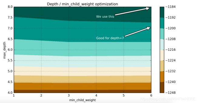
我们看到，从网格搜索的结果，分数的提高主要是基于max_depth增加. min_child_weight稍有影响的成绩，但是，我们看到，min_child_weight = 6会更好一些。

Step 3: 调节 gamma去降低过拟合风险

%%time

xgb_param_grid = {'gamma':[ 0.1 * i for i in range(0,5)]}

grid = GridSearchCV(XGBoostRegressor(eta=0.1, num_boost_round=50, max_depth=8, min_child_weight=6, colsample_bytree=0.5, subsample=0.5),
param_grid=xgb_param_grid, cv=5, scoring=mae_scorer)

grid.fit(train_x, train_y.values)

Wall time: 13min 45s

grid.grid_scores_, grid.best_params_, grid.best_score_

([mean: -1187.95975, std: 6.71340, params: {‘gamma’: 0.0},
mean: -1187.67788, std: 6.44332, params: {‘gamma’: 0.1},
mean: -1187.66616, std: 6.75004, params: {‘gamma’: 0.2},
mean: -1187.21835, std: 7.06771, params: {‘gamma’: 0.30000000000000004},
mean: -1188.35004, std: 6.50057, params: {‘gamma’: 0.4}],
{‘gamma’: 0.30000000000000004},
-1187.2183540791846)
我们选择使用偏小一些的 gamma.

Step 4: 调节样本采样方式 subsample 和 colsample_bytree

%%time

xgb_param_grid = {'subsample':[ 0.1 * i for i in range(6,9)],
                      'colsample_bytree':[ 0.1 * i for i in range(6,9)]}


grid = GridSearchCV(XGBoostRegressor(eta=0.1, gamma=0.2, num_boost_round=50, max_depth=8, min_child_weight=6),
                    param_grid=xgb_param_grid, cv=5, scoring=mae_scorer)
grid.fit(train_x, train_y.values)

Wall time: 28min 26s

grid.grid_scores_, grid.best_params_, grid.best_score_

([mean: -1185.67108, std: 5.40097, params: {‘colsample_bytree’: 0.6000000000000001, ‘subsample’: 0.6000000000000001},
mean: -1184.90641, std: 5.61239, params: {‘colsample_bytree’: 0.6000000000000001, ‘subsample’: 0.7000000000000001},
mean: -1183.73767, std: 6.15639, params: {‘colsample_bytree’: 0.6000000000000001, ‘subsample’: 0.8},
mean: -1185.09329, std: 7.04215, params: {‘colsample_bytree’: 0.7000000000000001, ‘subsample’: 0.6000000000000001},
mean: -1184.36149, std: 5.71298, params: {‘colsample_bytree’: 0.7000000000000001, ‘subsample’: 0.7000000000000001},
mean: -1183.83446, std: 6.24654, params: {‘colsample_bytree’: 0.7000000000000001, ‘subsample’: 0.8},
mean: -1184.43055, std: 6.68009, params: {‘colsample_bytree’: 0.8, ‘subsample’: 0.6000000000000001},
mean: -1183.33878, std: 5.74989, params: {‘colsample_bytree’: 0.8, ‘subsample’: 0.7000000000000001},
mean: -1182.93099, std: 5.75849, params: {‘colsample_bytree’: 0.8, ‘subsample’: 0.8}],
{‘colsample_bytree’: 0.8, ‘subsample’: 0.8},
-1182.9309918891634)

可视化

_, scores =  convert_grid_scores(grid.grid_scores_)
scores = scores.reshape(3,3)

plt.figure(figsize=(10,5))
cp = plt.contourf(xgb_param_grid['subsample'], xgb_param_grid['colsample_bytree'], scores, cmap='BrBG')
plt.colorbar(cp)
plt.title('Subsampling params tuning')
plt.annotate('Optimum', xy=(0.895, 0.6), xytext=(0.8, 0.695), arrowprops=dict(facecolor='black'))
plt.xlabel('subsample')
plt.ylabel('colsample_bytree')
plt.grid(True)
plt.show()

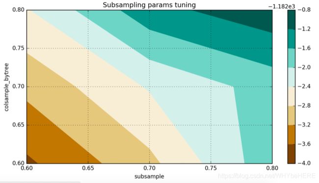
在当前的预训练模式的具体案例，我得到了下面的结果：
`{‘colsample_bytree’: 0.8, ‘subsample’: 0.8}, -1182.9309918891634)

Step 5: 减小学习率并增大树个数

5.1）50棵树

%%time
    
xgb_param_grid = {'eta':[0.5,0.4,0.3,0.2,0.1,0.075,0.05,0.04,0.03]} #由大到小选一些学习率
grid = GridSearchCV(XGBoostRegressor(num_boost_round=50, gamma=0.2, max_depth=8, min_child_weight=6,
                                        colsample_bytree=0.6, subsample=0.9),
                    param_grid=xgb_param_grid, cv=5, scoring=mae_scorer)

grid.fit(train_x, train_y.values)

CPU times: user 6.69 ms, sys: 0 ns, total: 6.69 ms
Wall time: 6.55 ms

grid.grid_scores_, grid.best_params_, grid.best_score_

([mean: -1205.85372, std: 3.46146, params: {‘eta’: 0.5},
mean: -1185.32847, std: 4.87321, params: {‘eta’: 0.4},
mean: -1170.00284, std: 4.76399, params: {‘eta’: 0.3},
mean: -1160.97363, std: 6.05830, params: {‘eta’: 0.2},
mean: -1183.66720, std: 6.69439, params: {‘eta’: 0.1},
mean: -1266.12628, std: 7.26130, params: {‘eta’: 0.075},
mean: -1709.15130, std: 8.19994, params: {‘eta’: 0.05},
mean: -2104.42708, std: 8.02827, params: {‘eta’: 0.04},
mean: -2545.97334, std: 7.76440, params: {‘eta’: 0.03}],
{‘eta’: 0.2},
-1160.9736284869114)
画图

eta, y = convert_grid_scores(grid.grid_scores_)
plt.figure(figsize=(10,4))
plt.title('MAE and ETA, 50 trees')
plt.xlabel('eta')
plt.ylabel('score')
plt.plot(eta, -y)
plt.grid(True)
plt.show()

{‘eta’: 0.2}, -1160.9736284869114 是目前最好的结果

这里0.1比0.2大

5.2）树的个数增加到100

xgb_param_grid = {'eta':[0.5,0.4,0.3,0.2,0.1,0.075,0.05,0.04,0.03]}
grid = GridSearchCV(XGBoostRegressor(num_boost_round=100, gamma=0.2, max_depth=8, min_child_weight=6,
                                        colsample_bytree=0.6, subsample=0.9),
                    param_grid=xgb_param_grid, cv=5, scoring=mae_scorer)

grid.fit(train_x, train_y.values)

CPU times: user 11.5 ms, sys: 0 ns, total: 11.5 ms
Wall time: 11.4 ms

grid.grid_scores_, grid.best_params_, grid.best_score_

([mean: -1231.04517, std: 5.41136, params: {‘eta’: 0.5},
mean: -1201.31398, std: 4.75456, params: {‘eta’: 0.4},
mean: -1177.86344, std: 3.67324, params: {‘eta’: 0.3},
mean: -1160.48853, std: 5.65336, params: {‘eta’: 0.2},
mean: -1152.24715, std: 5.85286, params: {‘eta’: 0.1},
mean: -1156.75829, std: 5.30250, params: {‘eta’: 0.075},
mean: -1184.88913, std: 6.08852, params: {‘eta’: 0.05},
mean: -1243.60808, std: 7.40326, params: {‘eta’: 0.04},
mean: -1467.04736, std: 8.70704, params: {‘eta’: 0.03}],
{‘eta’: 0.1},
-1152.2471498726127)

eta, y = convert_grid_scores(grid.grid_scores_)
plt.figure(figsize=(10,4))
plt.title('MAE and ETA, 100 trees')
plt.xlabel('eta')
plt.ylabel('score')
plt.plot(eta, -y)
plt.grid(True)
plt.show()

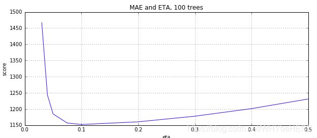
现在明显可见0.1比0.2小
增大了树的数量，学习率低一些的效果更好

5.3）200个树

%%time

xgb_param_grid = {'eta':[0.09,0.08,0.07,0.06,0.05,0.04]}
grid = GridSearchCV(XGBoostRegressor(num_boost_round=200, gamma=0.2, max_depth=8, min_child_weight=6,colsample_bytree=0.6, subsample=0.9), param_grid=xgb_param_grid, cv=5, scoring=mae_scorer)

grid.fit(train_x, train_y.values)

CPU times: user 21.9 ms, sys: 34 µs, total: 22 ms
Wall time: 22 ms

grid.grid_scores_, grid.best_params_, grid.best_score_

([mean: -1148.37246, std: 6.51203, params: {‘eta’: 0.09},
mean: -1146.67343, std: 6.13261, params: {‘eta’: 0.08},
mean: -1145.92359, std: 5.68531, params: {‘eta’: 0.07},
mean: -1147.44050, std: 6.33336, params: {‘eta’: 0.06},
mean: -1147.98062, std: 6.39481, params: {‘eta’: 0.05},
mean: -1153.17886, std: 5.74059, params: {‘eta’: 0.04}],
{‘eta’: 0.07},
-1145.9235944370419)

eta, y = convert_grid_scores(grid.grid_scores_)
plt.figure(figsize=(10,4))
plt.title('MAE and ETA, 200 trees')
plt.xlabel('eta')
plt.ylabel('score')
plt.plot(eta, -y)
plt.grid(True)
plt.show()

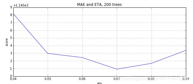
最终结果

%%time

# Final XGBoost model
bst = XGBoostRegressor(num_boost_round=200, eta=0.07, gamma=0.2, max_depth=8, min_child_weight=6, colsample_bytree=0.6, subsample=0.9)

cv = bst.kfold(train_x, train_y, nfold=5)

CPU times: user 1.26 ms, sys: 22 µs, total: 1.28 ms
Wall time: 1.07 ms

cv

test-mae-mean 1146.997852
test-mae-std 9.541592
train-mae-mean 1036.557251
train-mae-std 0.974437
Name: 199, dtype: float64

我们看到200棵树最好的ETA是0.07。正如我们所预料的那样，ETA和num_boost_round依赖关系不是线性的，但是有些关联。
们花了相当长的一段时间优化xgboost. 从初始值: 1219.57. 经过调参之后达到 MAE=1171.77.
我们还发现参数之间的关系ETA和num_boost_round：
100 trees, eta=0.1: MAE=1152.247
200 trees, eta=0.07: MAE=1145.92
`XGBoostRegressor(num_boost_round=200, gamma=0.2, max_depth=8, min_child_weight=6, colsample_bytree=0.6, subsample=0.9, eta=0.07).

笔记作分享和自己记录学习过程使用，如果内容有错误或问题，请各位朋友留言指出，多多评论^ ^。
参考内容：

• python数据分析与机器学习实战【2019新版】- XGBoost 调参实例https://edu.csdn.net/course/play/3904/300798
• XGBoost Tutorials：https://xgboost.readthedocs.io/en/latest/