[足式机器人]Part3 机构运动学与动力学分析与建模 Ch00-2(1) 质量刚体的在坐标系下运动

本文仅供学习使用，总结很多本现有讲述运动学或动力学书籍后的总结，从矢量的角度进行分析，方法比较传统，但更易理解，并且现有的看似抽象方法，两者本质上并无不同。

2024年底本人学位论文发表后方可摘抄
若有帮助请引用
本文参考：
黎 旭,陈 强 洪,甄 文 强 等.惯 性 张 量 平 移 和 旋 转 复 合 变 换 的 一 般 形 式 及 其 应 用[J].工 程 数 学 学 报,2022,39(06):1005-1011.

食用方法
质量点的动量与角动量
刚体的动量与角动量——力与力矩的关系
惯性矩阵的表达与推导——在刚体运动过程中的作用
惯性矩阵在不同坐标系下的表达
务必自己推导全部公式，并理解每个符号的含义

---

2. 质量刚体的在坐标系下运动

2.1 质量点 Mass Partical 的状态

对于质量点而言，其自身在笛卡尔坐标系中的状态仅包括运动状态。由热力学所引起自身的温度变化状态，由此产生的体积变化状态，或者自身亮度的状态变化等，都认为不会对运动状态产生干扰，即将某一空间实体等效为质量点，此时的笛卡尔坐标系所表示的状态空间就是三维空间。

由此，将质量点运动状态的改变视为力对质量点的作用：
$$F_{\mathrm{P}}^F=\frac{\mathrm{d}{p}_{\mathrm{P}}^F}{\mathrm{dt}}=\frac{\mathrm{d}\left(m{V}_{\mathrm{P}}^F\right)}{\mathrm{dt}}={\frac{\mathrm{d}m}{\mathrm{dt}}}_{\nearrow 0}{V}_{\mathrm{P}}^F+\frac{\mathrm{d}{V}_{\mathrm{P}}^F}{\mathrm{dt}}m=m{a}_{\mathrm{P}}^F$$
τ ⃗ P F = d h ⃗ P F d t = d ( m ⋅ R ⃗ P F × V ⃗ P F ) d t = d ( R ⃗ P F × V ⃗ P F ) d t m = [ ( d R ⃗ P F d t × V ⃗ P F ) ↗ 0 + R ⃗ P F × d V ⃗ P F d t ] m = R ⃗ P F × F ⃗ P F = R ⃗ P F × d p ⃗ P F d t \begin{split} \vec{\tau}_{\mathrm{P}}^{F}&=\frac{\mathrm{d}\vec{h}_{\mathrm{P}}^{F}}{\mathrm{dt}}=\frac{\mathrm{d}\left( m\cdot \vec{R}_{\mathrm{P}}^{F}\times \vec{V}_{\mathrm{P}}^{F} \right)}{\mathrm{dt}}=\frac{\mathrm{d}\left( \vec{R}_{\mathrm{P}}^{F}\times \vec{V}_{\mathrm{P}}^{F} \right)}{\mathrm{dt}}m \\ &=\left[ \left( \frac{\mathrm{d}\vec{R}_{\mathrm{P}}^{F}}{\mathrm{dt}}\times \vec{V}_{\mathrm{P}}^{F} \right) _{\nearrow 0}+\vec{R}_{\mathrm{P}}^{F}\times \frac{\mathrm{d}\vec{V}_{\mathrm{P}}^{F}}{\mathrm{dt}} \right] m=\vec{R}_{\mathrm{P}}^{F}\times \vec{F}_{\mathrm{P}}^{F}=\vec{R}_{\mathrm{P}}^{F}\times \frac{\mathrm{d}\vec{p}_{\mathrm{P}}^{F}}{\mathrm{dt}} \end{split} τ PF​​=dtdh PF​​=dtd(m⋅R PF​×V PF​)​=dtd(R PF​×V PF​)​m= ​(dtdR PF​​×V PF​)↗0​+R PF​×dtdV PF​​ ​m=R PF​×F PF​=R PF​×dtdp ​PF​​​

如果说动量是表述物体运动状态的量，那么角动量就是描述物体旋转状态的量；如果说力是改变物体运动状态的量，那么扭矩就是改变物体旋转状态的量。

认为质量点的质量不发生改变：

• 质量点的动量Linear Momentum：$p_{\mathrm{P}}^F$——点 $P$ 在固定坐标系$\left\{F\right\}$下的动量参数 $$p_{\mathrm{P}}^F=m{V}_{\mathrm{P}}^F$$
• 质量点的角动量Angular Momentum：$h_{\mathrm{P}/\mathrm{O}}^F$——点 $P$ 在固定坐标系$\left\{F\right\}$下，相对于点 $O$ 的角动量参数（又可称为动量矩）
  $h_{\mathrm{P}/\mathrm{O}}^F=R_{\mathrm{OP}}^F\times p_{\mathrm{P}}^F=R_{\mathrm{OP}}^F\times \left(m{V}_{\mathrm{P}}^F\right)=m\cdot \left(R_{\mathrm{P}}^F-R_{\mathrm{O}}^F\right)\times V_{\mathrm{P}}^F=h_{\mathrm{P}}^F-m\cdot R_{\mathrm{O}}^F\times V_{\mathrm{P}}^F$

其中，动量的计算是依据固定坐标系进行描述的，而角动量通常与所选择的运动坐标系有关。令 $O$ 为固定坐标系中任意一参考点，此时以点 $O$ 计算点 $P$ 的扭矩${\tau }_{\mathrm{P}/\mathrm{O}}^F$为:
$$\begin{array}{rl}{\tau }_{\mathrm{P}/\mathrm{O}}^F& =R_{\mathrm{OP}}^F\times F_{\mathrm{P}}^F=R_{\mathrm{OP}}^F\times \frac{\mathrm{d}{p}_{\mathrm{P}}^F}{\mathrm{dt}}=\frac{\mathrm{d}\left(R_{\mathrm{OP}}^F\times p_{\mathrm{P}}^F\right)}{\mathrm{dt}}-\frac{\mathrm{d}\left(R_{\mathrm{OP}}^F\right)}{\mathrm{dt}}\times p_{\mathrm{P}}^F\\ & =\frac{\mathrm{d}\left(R_{\mathrm{OP}}^F\times p_{\mathrm{P}}^F\right)}{\mathrm{dt}}-\frac{\mathrm{d}\left(R_{\mathrm{P}}^F-R_{\mathrm{O}}^F\right)}{\mathrm{dt}}\times p_{\mathrm{P}}^F=\frac{\mathrm{d}{h}_{\mathrm{P}/\mathrm{O}}^F}{\mathrm{dt}}+V_{\mathrm{O}}^F\times p_{\mathrm{P}}^F\end{array}$$

由上式可知，当$V_{\mathrm{O}}^F\parallel V_{\mathrm{P}}^F$（特别是$O$与$P$为同一点）时，或$V_{\mathrm{O}}^F=0$（相当于坐标系下一定点）时，有：${\tau }_{\mathrm{P}}^O=\frac{\mathrm{d}{h}_{\mathrm{P}}^O}{\mathrm{dt}}$

此时，已知：$R_{\mathrm{OP}}^F\times \frac{\mathrm{d}\left(m{V}_{\mathrm{P}}^F\right)}{\mathrm{d}t}=R_{\mathrm{OP}}^F\times F_{\mathrm{P}}^F$，对$h_{\mathrm{P}/\mathrm{O}}^F$求导，则有：
$$\begin{array}{rl}\frac{\mathrm{d}{h}_{\mathrm{P}/\mathrm{O}}^F}{\mathrm{d}t}& =\frac{\mathrm{d}{R}_{\mathrm{OP}}^F}{\mathrm{d}t}\times p_{\mathrm{P}}^F+R_{\mathrm{OP}}^F\times \frac{\mathrm{d}{p}_{\mathrm{P}}^F}{\mathrm{d}t}=m\cdot \frac{\mathrm{d}{R}_{\mathrm{OP}}^F}{\mathrm{d}t}\times V_{\mathrm{P}}^F+m\cdot R_{\mathrm{OP}}^F\times \frac{\mathrm{d}{V}_{\mathrm{P}}^F}{\mathrm{d}t}\\ & =m\cdot \frac{\mathrm{d}\left(R_{\mathrm{P}}^F-R_{\mathrm{O}}^F\right)}{\mathrm{d}t}\times V_{\mathrm{P}}^F+m\cdot R_{\mathrm{OP}}^F\times \frac{\mathrm{d}{V}_{\mathrm{P}}^F}{\mathrm{d}t}\\ & =m\cdot \frac{\mathrm{d}\left(R_{\mathrm{P}}^F-R_{\mathrm{O}}^F\right)}{\mathrm{d}t}\times V_{\mathrm{P}}^F+R_{\mathrm{OP}}^F\times F_{\mathrm{P}}^F\end{array}$$

可见，同上所述：当$V_{\mathrm{O}}^F=0$时，即$\frac{\mathrm{d}{h}_{\mathrm{P}/\mathrm{O}}^F}{\mathrm{d}t}=m\cdot \left(V_{\mathrm{P}}^F-{V_{\mathrm{O}}^F}_{\nearrow 0}\right)\times V_{\mathrm{P}}^F+R_{\mathrm{OP}}^F\times F_{\mathrm{P}}^F=R_{\mathrm{OP}}^F\times F_{\mathrm{P}}^F$；当$V_{\mathrm{O}}^F\parallel V_{\mathrm{P}}^F$时，即$\frac{\mathrm{d}{h}_{\mathrm{P}/\mathrm{O}}^F}{\mathrm{d}t}={\left(m\cdot \left(V_{\mathrm{P}}^F-V_{\mathrm{O}}^F\right)\times V_{\mathrm{P}}^F\right)}_{\nearrow 0}+R_{\mathrm{OP}}^F\times F_{\mathrm{P}}^F=R_{\mathrm{OP}}^F\times F_{\mathrm{P}}^F$。

因此，对于质点对某定点的动量矩对时间的一阶导数，等于作用力对该定点的矩，即为质点的动量矩定理:
$$\frac{\mathrm{d}{h}_{\mathrm{P}/{\mathrm{O}}_{\mathrm{Fixed}}}^F}{\mathrm{d}t}=R_{{\mathrm{O}}_{\mathrm{Fixed}}\mathrm{P}}^F\times F_{\mathrm{P}}^F$$

例子1：球杆模型

$$\begin{array}{rl}{V}_{\mathrm{P}}^F& =\dot{r}{X}_{\mathrm{r}}+r\dot{\theta }{X}_{\theta }\\ a_{\mathrm{P}}^F& =\left(\ddot{r}-r{\dot{\theta }}^2\right)X_{\mathrm{r}}+\left(2\dot{r}\dot{\theta }\right)X_{\theta }\end{array}$$
$$\begin{array}{rl}{h}_{\mathrm{P}}^F& =R_{\mathrm{P}}^F\times p_{\mathrm{P}}^F=r{X}_{\mathrm{r}}\times \left(\dot{r}{X}_{\mathrm{r}}+r\dot{\theta }{X}_{\theta }\right)\cdot m=m{r}^2\dot{\theta }\hat{K}\\ {\tau }_{\mathrm{P}}^F& =\frac{\mathrm{d}{h}_{\mathrm{P}}^F}{\mathrm{dt}}=2m\dot{r}\dot{\theta }\hat{K}=R_{\mathrm{P}}^F\times F_{\mathrm{P}}^F=\left(r{X}_{\mathrm{r}}\right)\times \left(\left(\ddot{r}-r{\dot{\theta }}^2\right)X_{\mathrm{r}}+\left(2\dot{r}\dot{\theta }\right)X_{\theta }\right)\cdot m\\ & =R_{\mathrm{P}}^F\times \left(2\dot{r}\dot{\theta }\right)X_{\theta }\cdot m\end{array}$$
从受力分析的角度来看，小球仅受到了垂直于杆方向的支撑力作用，而在沿杆方向并没有力的作用，但根据小球的加速度方程(\ref{eq:ballrank1})可知，小球具有沿杆方向的运动。前者的描述是基于固定坐标系进行分析，而后者的描述是基于运动坐标系进行的分析，因此两者本质上没有矛盾关系。所谓的科氏加速度与向心力都是在运动坐标系下描述时，由于运动标架的不同，所产生的虚拟力，在实际的固定坐标系中也不参与功的作用。

2.2 运动刚体的状态

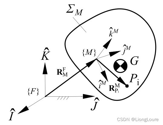
对于运动刚体${\Sigma }_{\mathrm{M}}$而言，需要将其上任意一点$P_{\mathrm{i}}$在固定坐标系$\left\{F:\left(\hat{I},\hat{J},\hat{K}\right)\right\}$下进行表述。而对于有质量的刚体而言，其最特殊的点就是其等效的质量中心，称为其为质心点 $G$ 或 $CoM$(center of mass)。

2.2.1 刚体的质心Center of Mass——点$G$或点$CoM$

$$m_{\mathrm{total}}\cdot R_{\mathrm{G}}^F=\sum m_{\mathrm{i}}\cdot R_{{\mathrm{P}}_{\mathrm{i}}}^F$$
对于刚体Rigid Body而言，其可视为 $N$ 个质量点的集合，并具有有限体积，且各质量点之间的距离为定值，即：
$$\Vert r_{\mathrm{i}}-r_{\mathrm{j}}\Vert =C_{\mathrm{ij}}i,j\in \left\{1,\cdots ,N\right\}$$
其中，$r_{\mathrm{i}}\in {\mathbb{R}}^3$为位置参数，$C_{\mathrm{ij}}\in \mathbb{R}$为距离参数。

刚体在现实中并不存在，只是一种近似，且有：${\omega }_{\mathrm{Flex}}\gg {\omega }_{\mathrm{RB}}=0$。刚体的自然频率Nature Frequency为0，柔性体Flexible Body的自然频率远大于刚体的自然频率。

质量点在空间坐标系中只需要对位置Position进行表征Configurate，而刚体还需要对其姿态Pose进行描述

考虑质量点的动量与角动量方程，首先考虑运动刚体的角动量与动量方程：
$$\{\begin{array}{l}{P}_{\mathrm{G}}^F=m_{\mathrm{total}}{V}_{\mathrm{G}}^F\\ H_{{\Sigma }_{\mathrm{M}}/\mathrm{O}}^F={\sum }_i^N{R}_{{\mathrm{OP}}_{\mathrm{i}}}^F\times P_{{\mathrm{P}}_{\mathrm{i}}}^F={\sum }_i^N{h}_{{\mathrm{P}}_{\mathrm{i}}/\mathrm{O}}^F\end{array}$$

2.2.2 刚体的动量矩定理 theorem of moment of momentum

对于运动刚体上一微元点${\mathrm{P}}_{\mathrm{i}}$进行力矩分析，则有：
$$\begin{array}{rl}& H_{{\Sigma }_{\mathrm{M}}/\mathrm{O}}^F=\sum _i^N{h}_{{\mathrm{P}}_{\mathrm{i}}/\mathrm{O}}^F=\int h_{{\mathrm{P}}_{\mathrm{i}}/\mathrm{O}}^F=\int R_{{\mathrm{OP}}_{\mathrm{i}}}^F\times \left(\mathrm{d}{m}_i\cdot \frac{\mathrm{d}{R}_{{\mathrm{P}}_{\mathrm{i}}}^F}{\mathrm{d}t}\right)\\ \Rightarrow \frac{\mathrm{d}{H}_{{\Sigma }_{\mathrm{M}}/\mathrm{O}}^F}{\mathrm{d}t}& =\frac{\mathrm{d}\left(\int R_{{\mathrm{OP}}_{\mathrm{i}}}^F\times \left(\mathrm{d}{m}_i\cdot \frac{\mathrm{d}{R}_{{\mathrm{P}}_{\mathrm{i}}}^F}{\mathrm{d}t}\right)\right)}{\mathrm{d}t}=\int \left(R_{{\mathrm{OP}}_{\mathrm{i}}}^F\times \left(\mathrm{d}{m}_i\cdot a_{{\mathrm{P}}_{\mathrm{i}}}^F\right)\right)+\int \left(\left(V_{{\mathrm{P}}_{\mathrm{i}}}^F-V_{\mathrm{O}}^F\right)\times \left(\mathrm{d}{m}_i\cdot V_{{\mathrm{P}}_{\mathrm{i}}}^F\right)\right)\\ & =\int \left(R_{{\mathrm{OP}}_{\mathrm{i}}}^F\times F_{{\mathrm{P}}_{\mathrm{i}}}^F\right)-\int \left(V_{\mathrm{O}}^F\times \left(\mathrm{d}{m}_i\cdot V_{{\mathrm{P}}_{\mathrm{i}}}^F\right)\right)=M_{{\Sigma }_{\mathrm{M}}/\mathrm{O}}^F-V_{\mathrm{O}}^F\times P_{{\Sigma }_{\mathrm{M}}}^F\end{array}$$

若参考点$O$为固定坐标系下一固定点，则上式简化为：
$$\frac{\mathrm{d}{H}_{{\Sigma }_{\mathrm{M}}/{\mathrm{O}}_{\mathrm{Fixed}}}^F}{\mathrm{d}t}=M_{{\Sigma }_{\mathrm{M}}/{\mathrm{O}}_{\mathrm{Fixed}}}^F$$