深度学习入门——深层神经网络模型的模块搭建

深层神经网络模型的搭建

学习记录自：deeplearning.ai-andrewNG-master

L层神经网络模型概览

该模型可以总结为：[LINEAR -> RELU] × (L-1) -> LINEAR -> SIGMOID。
详细结构：
• 输入维度为（64,64,3）的图像，将其展平为大小为（12288,1）的向量。
• 相应的向量：[x0,x1,…,x12287]T乘以权重矩阵W[1]，然后加上截距b[1]，结果为线性单位。
• 接下来计算获得的线性单元。对于每个(W[l],b[l])，可以重复数次，具体取决于模型体系结构。
• 最后，采用最终线性单位的sigmoid值。如果大于0.5，则将其分类为猫。
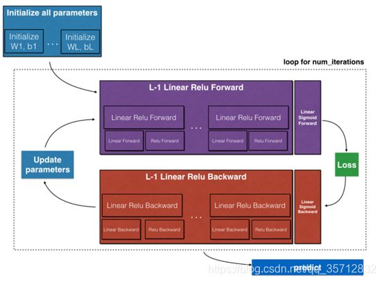
通用步骤：
与往常一样，将遵循深度学习步骤来构建模型：
1.初始化参数/定义超参数
2.循环num_iterations次：
a. 正向传播
b. 计算损失函数
C. 反向传播
d. 更新参数（使用参数和反向传播的梯度）
4.使用训练好的参数来预测标签

L层神经网络各隐藏层维度关系

更深的L层神经网络的初始化更加复杂，因为存在更多的权重矩阵和偏差向量。 完成 initialize_parameters_deep后，应确保各层之间的维度匹配。下面以输入的X大小为（12288，209），样本数为209为例，给出各层神经元个数关系。

正向传播模块与反向传播模块

传播模块包括线性计算部分、线性激活部分以及整合到L层模型部分。概览图如下示：

对于正向传播，前L-1层均为Relu函数激活，对于整个模型而言，需要重复计算Relu函数L-1次。把单次的Linear->Relu重复L-1次即可。
对于反向传播，从后往前进行计算，只需要把Relu->Linear重复L-1次即可，需要注意的是反向传播中会用到正向传播中的缓存值。
上述传播计算如下图所示：

图 1 正向传播模型

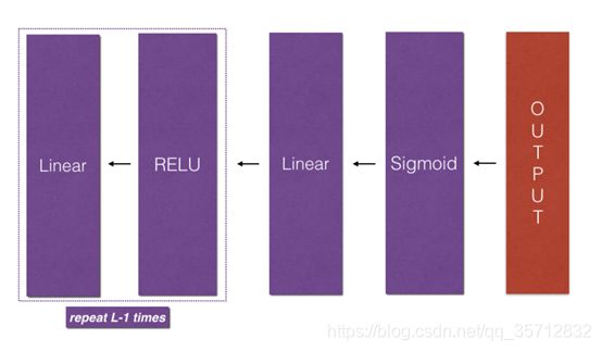
图2反向传播模型

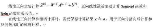
线性正向与正向线性激活

线性反向与反向线性激活

图 3 反向传播时的梯度计算图

上述计算公式如下：

图 4反向传播梯度计算公式

参数更新

模型的优化伴随参数更新，这里L层神经网络模型的参数更新采用基于梯度下降的更新。

本文的Deep neural network 模型如下

DNN模块–代码

"""
    构建一个深层神经网络；各个模块的搭建
"""
#首先本次 模块搭建需要的包
import numpy as np
import h5py
import matplotlib.pyplot as plt
from dnn_utils_v2 import sigmoid, sigmoid_backward, relu, relu_backward  #辅助函数

#初始化一个2层的 神经网络模型 初始参数
def initialize_parameters(n_x, n_h, n_y):
    """
    Argument:
    n_x -- 输入层的大小
    n_h -- 隐藏层的大小
    n_y -- 输出层的大小
    
    返回值：
    parameters --整合到字典里 进行返回
                    W1 -- weight matrix of shape (n_h, n_x)
                    b1 -- bias vector of shape (n_h, 1)
                    W2 -- weight matrix of shape (n_y, n_h)
                    b2 -- bias vector of shape (n_y, 1)
    """
    
    W1 = np.random.randn(n_h, n_x)*0.01
    b1 = np.zeros((n_h,1))
    W2 = np.random.randn(n_y, n_h)*0.01
    b2 = np.zeros(n_y,1)
    
    
    assert(W1.shape == (n_h, n_x))
    assert(b1.shape == (n_h, 1))
    assert(W2.shape == (n_y, n_h))
    assert(b2.shape == (n_y, 1))
    
    parameters = {"W1": W1,
                  "b1": b1,
                  "W2": W2,
                  "b2": b2}
    
    return parameters    


#初始化一个具有L层的神经网络初始参数  
"""
利用 layer_dims 来存储每一层的单元数 如: [2 , , , , 1]
关键为 每一层的权重矩阵维度为    Wl-- (layer_dims[l], layer_dims[l-1])
                              bl-- (layer_dims[l], 1)
"""
def initialize_parameters_deep(layer_dims):
    """
    layer_dims -- 包含该神经网络的层数  以及每一层的单元数
    
    返回值:
    parameters -- 每一层的权重参数w b  : "W1", "b1", ..., "WL", "bL":
                    Wl -- weight matrix of shape (layer_dims[l], layer_dims[l-1])
                    bl -- bias vector of shape (layer_dims[l], 1)
    """
    
    parameters = {}
    L = len(layer_dims)            # 读取该神经网络的层数

    #初始化每一层的权重参数
    for l in range(1, L):
        
        parameters['W' + str(l)] = np.random.randn(layer_dims[l],layer_dims[l-1])*0.01
        parameters['b' + str(l)] = np.zeros((layer_dims[l],1))
        
        assert(parameters['W' + str(l)].shape == (layer_dims[l], layer_dims[l-1]))
        assert(parameters['b' + str(l)].shape == (layer_dims[l], 1))

        
    return parameters
    


#神经神经网络的正向传播 
"""
分为三个部分
        LINEAR (计算 z = w*x+b)
        LINEAR -> ACTIVATION，其中激活函数采用ReLU或Sigmoid。(计算g(z))
        [LINEAR -> RELU]  (L-1) -> LINEAR -> SIGMOID（整个模型） (计算整个模型正向传播过程中的 Z 与 g(Z))
"""
 ##线性正向传播
def linear_forward(A, W, b):
   """
   线性正向传播 未激活的值

   Arguments:
   A -- 上一层的激活值 (或者是输入): (size of previous layer, number of examples)
   W -- 权重参数  维度：(size of current layer, size of previous layer)
   b -- 参数  维度： (size of the current layer, 1)

   Returns:
   Z -- 激活前的值  
   cache -- 暂存信息 (反向传播时用)  利用字典存储："A", "W" and "b" 
   """
   
   Z = np.dot(W,A) + b
   
   assert(Z.shape == (W.shape[0], A.shape[1]))
   #暂存 cache
   cache = (A, W, b)
   
   return Z, cache   
    
 ##正向线性激活函数    用于辅助 L层模型激活
def linear_activation_forward(A_prev, W, b, activation):
    """
    计算激活函数值

    Arguments:
    A_prev -- 本一层的输入值(上一层的激活函数值): (size of previous layer, number of examples)
    W -- 维度： (size of current layer, size of previous layer)
    b -- 维度：(size of the current layer, 1)
    activation -- 存储本神经网络中用到的 激活函数: "sigmoid" or "relu"

    返回值:
    A -- 计算后的本层的激活函数值
    cache -- 暂存值 A
    """
    
    if activation == "sigmoid":
        # Inputs: "A_prev, W, b". Outputs: "A, activation_cache".
        Z, linear_cache = linear_forward(A_prev,W,b)
        A, activation_cache = sigmoid(Z)
    
    elif activation == "relu":
        # Inputs: "A_prev, W, b". Outputs: "A, activation_cache".
        Z, linear_cache = linear_forward(A_prev,W,b)
        A, activation_cache = relu(Z)
    
    assert (A.shape == (W.shape[0], A_prev.shape[1]))
    cache = (linear_cache, activation_cache)

    return A, cache

 ##正向传播时的模型   用于方便计算整个神经网络中的  激活函数值  同时暂存大量信息
"""
        基于先前编写的函数
        使用for循环复制[LINEAR-> RELU]（L-1）次
        在“cache”列表中更新缓存。 要将新值 c添加到list中，可以使用list.append(c)
"""
def L_model_forward(X, parameters):
    """
    实现l-1层的RELU激活值计算 以及 第L层的sigmoid激活值计算 [LINEAR->RELU]*(L-1)->LINEAR->SIGMOID computation
    
    Arguments:
    X -- data, numpy array of shape (input size, number of examples)
    parameters -- 初始化参数
    
    返回值:
    AL --记录上一层的 激活函数值 
    caches -- list of caches containing:
                every cache of linear_relu_forward() (there are L-1 of them, indexed from 0 to L-2)
                the cache of linear_sigmoid_forward() (there is one, indexed L-1)
    """

    caches = []
    A = X
    L = len(parameters) // 2                  # 神经网络层数
    
    # 实现L-1层的正向传播线性激活函数计算 
    for l in range(1, L):
        A_prev = A   #记录上一层的激活函数值  用于本层计算

        A, cache = linear_activation_forward(A_prev,parameters['W' + str(l)],parameters['b' + str(l)],activation = "relu")
        caches.append(cache)
        #每一层的数据（A)暂存   进入caches
    
    # 计算输出值 sigmoid()
    AL, cache = linear_activation_forward(A,parameters['W' + str(L)],parameters['b' + str(L)],activation = "sigmoid")
    caches.append(cache)
    
    assert(AL.shape == (1,X.shape[1]))  #最后验证维度的正确性
            
    return AL, caches
    


#损失函数的计算
def compute_cost(AL, Y):
    """
    实现损失计算

    Arguments:
    AL -- probability vector corresponding to your label predictions, shape (1, number of examples)
    Y -- true "label" vector (for example: containing 0 if non-cat, 1 if cat), shape (1, number of examples)

    Returns:
    cost -- cross-entropy cost
    """
    
    m = Y.shape[1]  #记录样本个数

    #利用已经得到的AL(所有样本在神经网络中的输出值) 和 Y  计算 损失
   
    cost = -1 / m * np.sum(Y * np.log(AL) + (1-Y) * np.log(1-AL),axis=1,keepdims=True)
    
    
    cost = np.squeeze(cost)      # 保证得到的值是一个矩阵
    assert(cost.shape == ())
    
    return cost


#反向传播  反向传播用于计算损失函数相对于参数的梯度
"""
分为三个部分
        LINEAR backward  (z = w*a+b)  计算z 对 w b a的导数
        LINEAR -> ACTIVATION backward，其中激活函数使用ReLU或sigmoid 的导数计算
        [LINEAR -> RELU]  (L-1) -> LINEAR -> SIGMOID backward（整个模型）     
"""

  ##线性反向
def linear_backward(dZ, cache):
    """
    每一层对前一层的导数计算
    Arguments:
    dZ -- 后一层对前一层的导数dz (of current layer l)
    cache -- tuple of values (A_prev, W, b) coming from the forward propagation in the current layer

    返回值:
    dA_prev -- 对下一层的导数 即 dA (of the previous layer l-1), same shape as A_prev
    dW -- Gradient of the cost with respect to W (current layer l), same shape as W
    db -- Gradient of the cost with respect to b (current layer l), same shape as b
    """
    
    #从正向传播过程中的 cache中读取  w b A的信息
    A_prev, W, b = cache
    m = A_prev.shape[1]
   
    dW = 1 / m * np.dot(dZ ,A_prev.T)
    db = 1 / m * np.sum(dZ,axis = 1 ,keepdims=True)
    dA_prev = np.dot(W.T,dZ) 
    
    
    assert (dA_prev.shape == A_prev.shape)
    assert (dW.shape == W.shape)
    assert (db.shape == b.shape)
    
    return dA_prev, dW, db


   ##线性反向激活 (包含激活函数之后的导数值计算)
def linear_activation_backward(dA, cache, activation):
    """
    实现线性 -> 激活层的反向传播
    
    Arguments:
    dA -- 线性反向时计算得到的 dA 
    cache -- 元组数据 (linear_cache, activation_cache) 
    activation -- 神经网络中用到的激活函数
    
    Returns:
    dA_prev -- Gradient of the cost with respect to the activation (of the previous layer l-1), same shape as A_prev
    dW -- Gradient of the cost with respect to W (current layer l), same shape as W
    db -- Gradient of the cost with respect to b (current layer l), same shape as b
    """
    linear_cache, activation_cache = cache
    
    if activation == "relu":
        
        dZ = relu_backward(dA, activation_cache)  #dz = dA*1
        dA_prev, dW, db = linear_backward(dZ, linear_cache)
        
        
    elif activation == "sigmoid":
        
        dZ = sigmoid_backward(dA, activation_cache) #dz = dA*sigmoid'(z)
        dA_prev, dW, db = linear_backward(dZ, linear_cache)
        
    
    return dA_prev, dW, db


  ##反向L层模型
"""
  从L层开始向后遍历所有隐藏层   将L层的缓存值 传播到L-1层
  计算得到所有层   损失函数对 a w b 的导数
  实现   sigmoid->linear->[Relu->linear]
                             repeat L-1 times
"""
def L_model_backward(AL, Y, caches):
    """
    实现反向传播 [LINEAR->RELU] * (L-1) -> LINEAR -> SIGMOID group

    Arguments:
    AL -- probability vector, output of the forward propagation (L_model_forward())
    Y -- true "label" vector (containing 0 if non-cat, 1 if cat)
    caches -- 每一层在正向传播时的缓存值:
                every cache of linear_activation_forward() with "relu" (it's caches[l], for l in range(L-1) i.e l = 0...L-2)
                the cache of linear_activation_forward() with "sigmoid" (it's caches[L-1])
    
    返回值:
    grads -- A dictionary with the gradients
             grads["dA" + str(l)] = ...
             grads["dW" + str(l)] = ...
             grads["db" + str(l)] = ...
    """
    grads = {}
    L = len(caches) # 神经网络层数
    m = AL.shape[1]
    Y = Y.reshape(AL.shape) # 保证Y 与AL的维度一致

    # 初始化反向传播
    
    dAL = - (np.divide(Y, AL) - np.divide(1 - Y, 1 - AL))
  
    
    # 第一层 (SIGMOID -> LINEAR) gradients. Inputs: "AL, Y, caches". Outputs: "grads["dAL"], grads["dWL"], grads["dbL"]
    
    current_cache = caches[L-1]   #读取信息
    grads["dA" + str(L)], grads["dW" + str(L)], grads["db" + str(L)] = linear_activation_backward(dAL, current_cache, activation = "sigmoid")
   
      
    #遍历从1 - L-1 的反向传播     Relu->linear->Relu->linear->.....
    for l in reversed(range(L - 1)):
        # lth layer: (RELU -> LINEAR) gradients.
        # Inputs: "grads["dA" + str(l + 2)], caches". Outputs: "grads["dA" + str(l + 1)] , grads["dW" + str(l + 1)] , grads["db" + str(l + 1)] 
        
        current_cache = caches[l]
        dA_prev_temp, dW_temp, db_temp = linear_activation_backward(grads["dA" + str(l+2)], current_cache, activation = "relu")
        grads["dA" + str(l + 1)] = dA_prev_temp
        grads["dW" + str(l + 1)] = dW_temp
        grads["db" + str(l + 1)] = db_temp
        


    return grads




#参数更新
def update_parameters(parameters, grads, learning_rate):
   """
   利用梯度下降进行 参数更新
   
   Arguments:
   parameters -- 参数字典
   grads -- 梯度字典
   
   返回值:
   parameters -- 新的参数字典 
                 parameters["W" + str(l)] = ... 
                 parameters["b" + str(l)] = ...
   """
   
   L = len(parameters) // 2 # 神经网络层数

   # 利用学习率 和梯度 进行更新
  
   for l in range(L):
       parameters["W" + str(l+1)] =  parameters["W" + str(l+1)] - learning_rate * grads["dW" + str(l + 1)]
       parameters["b" + str(l+1)] = parameters["b" + str(l+1)] - learning_rate * grads["db" + str(l + 1)]

       
   return parameters 

代码中的dnn_utils_v2 是自己写的模块完成激活函数值的计算以及梯度的辅助计算。

利用上述模块函数可以得到一个简单的DNN参数训练器

def L_layer_model(X, Y, layers_dims, learning_rate = 0.0075, num_iterations = 3000, print_cost=False):
    """
    实现L层神经网络 [LINEAR->RELU]*(L-1)->LINEAR->SIGMOID.
    
    Arguments:
    X -- data, numpy array of shape (number of examples, num_px * num_px * 3)
    Y -- true "label" vector (containing 0 if cat, 1 if non-cat), of shape (1, number of examples)
    layers_dims -- 神经网络各层单元数   大小 (number of layers + 1) 如:layers_dims = [12288, 20, 7, 5, 1]
    learning_rate -- 参数更新率
    num_iterations -- 迭代次数
    print_cost -- if True, it prints the cost every 100 steps
    
    返回值:
    parameters -- 返回模型训练后的参数
    """

    costs = []                         # 损失值 初始化为一个矩阵
    
    #参数初始化

    parameters = initialize_parameters_deep(layers_dims)

    
    # 梯度下降 进行训练优化
    for i in range(0, num_iterations):

        # 正向传播: [LINEAR -> RELU]*(L-1) -> LINEAR -> SIGMOID.
     
        AL, caches = L_model_forward(X, parameters)
 
        # 损失函数
        
        cost = compute_cost(AL, Y)
        
        # 反向传播
        
        grads = L_model_backward(AL, Y, caches)
        
        # 参数更新
        
        parameters = update_parameters(parameters, grads, learning_rate)
        
      return parameters