利用Python进行数据分析的学习笔记——chap10

时间序列

日期和时间数据类型及工具

from datetime import datetime
now = datetime.now()
now

datetime.datetime(2022, 3, 4, 8, 23, 31, 842698)

now.year,now.month,now.day

(2022, 3, 4)

#时间差
delta = datetime(2022,3,3)-datetime(1998,10,20,8,10)
delta

datetime.timedelta(days=8534, seconds=57000)

delta.days

delta.seconds

from datetime import timedelta
start = datetime(2022,3,3)
start + timedelta(12)

datetime.datetime(2022, 3, 15, 0, 0)

start - 2*timedelta(12)

datetime.datetime(2022, 2, 7, 0, 0)

#有个知识点
import matplotlib.pyplot as plt
from pylab import *
img = plt.imread('datetime模块中的数据类型.png')
imshow(img)

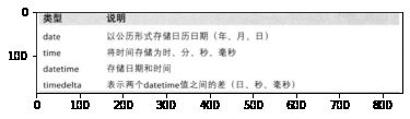
字符串和datetime的相互转换

stamp = datetime.datetime(2022,3,3)
str(stamp)

'2022-03-03 00:00:00'

stamp.strftime('%Y-%m-%d')

'2022-03-03'

#有个知识点
import matplotlib.pyplot as plt
from pylab import *
img = plt.imread('datetime格式定义.png')
imshow(img)

value = '2022-03-03'
#strptime将字符串转换成日期
datetime.datetime.strptime(value,'%Y-%m-%d')

datetime.datetime(2022, 3, 3, 0, 0)

datestrs = ['7/6/2022','8/6/2022']
[datetime.datetime.strptime(x,'%m/%d/%Y') for x in datestrs]

[datetime.datetime(2022, 7, 6, 0, 0), datetime.datetime(2022, 8, 6, 0, 0)]

from dateutil.parser import parse
parse('2022-03-03')

datetime.datetime(2022, 3, 3, 0, 0)

parse('Jan 31,1997 10:45 PM')

datetime.datetime(2022, 1, 31, 22, 45)

parse('6/12/2011',dayfirst=True)

datetime.datetime(2011, 12, 6, 0, 0)

import pandas as pd
pd.to_datetime(datestrs)

DatetimeIndex(['2022-07-06', '2022-08-06'], dtype='datetime64[ns]', freq=None)

idx = pd.to_datetime(datestrs + [None])
idx

DatetimeIndex(['2022-07-06', '2022-08-06', 'NaT'], dtype='datetime64[ns]', freq=None)

idx[2]#Not a Time是pandas中时间戳数据的NA值

NaT

pd.isnull(idx)

array([False, False,  True])

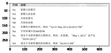
#有个知识点
import matplotlib.pyplot as plt
from pylab import *
img = plt.imread('特定于当前环境的日期格式.png')
imshow(img)

时间序列基础

from datetime import datetime
from pandas import DataFrame, Series
dates = [datetime(2011,1,2),datetime(2011,1,5),datetime(2011,1,7),
        datetime(2011,1,8),datetime(2011,1,10),datetime(2011,1,12)]
ts = Series(np.random.randn(6),index=dates)
ts

2011-01-02    0.955968
2011-01-05   -3.053080
2011-01-07   -0.724017
2011-01-08   -1.219987
2011-01-10   -0.303126
2011-01-12   -0.979242
dtype: float64

type(ts)

pandas.core.series.Series

ts.index

DatetimeIndex(['2011-01-02', '2011-01-05', '2011-01-07', '2011-01-08',
               '2011-01-10', '2011-01-12'],
              dtype='datetime64[ns]', freq=None)

#不同索引的时间序列之间的算术运算会自动按日期对齐
ts + ts[::2]

2011-01-02    1.911936
2011-01-05         NaN
2011-01-07   -1.448034
2011-01-08         NaN
2011-01-10   -0.606251
2011-01-12         NaN
dtype: float64

ts.index.dtype

dtype('


stamp = ts.index[0]
stamp

Timestamp('2011-01-02 00:00:00')

索引、选取、子集构造
stamp = ts.index[2]
ts[stamp]

-0.7240168825490924

ts['1/10/2011']

-0.30312563460424696

ts['20110110']

-0.30312563460424696

longer_ts = Series(np.random.randn(1000),
                  index=pd.date_range('1/1/2000',periods=1000))
longer_ts

2000-01-01   -0.238369
2000-01-02    1.119693
2000-01-03    0.092546
2000-01-04    1.110926
2000-01-05    0.170824
                ...   
2002-09-22   -0.468025
2002-09-23    0.260535
2002-09-24   -1.058960
2002-09-25    0.485363
2002-09-26   -0.593321
Freq: D, Length: 1000, dtype: float64

longer_ts['2001']

2001-01-01    0.333511
2001-01-02    0.669764
2001-01-03   -1.459111
2001-01-04    0.316825
2001-01-05   -0.949078
                ...   
2001-12-27   -1.992184
2001-12-28    0.062251
2001-12-29    0.750101
2001-12-30   -0.673639
2001-12-31   -1.512151
Freq: D, Length: 365, dtype: float64

longer_ts['2001-05']

2001-05-01    1.023397
2001-05-02    0.320480
2001-05-03   -0.518482
2001-05-04   -1.238117
2001-05-05   -0.295051
2001-05-06    1.482434
2001-05-07    0.034568
2001-05-08   -1.260276
2001-05-09    0.661322
2001-05-10    1.838568
2001-05-11    0.978017
2001-05-12    1.347121
2001-05-13    0.665021
2001-05-14   -2.233556
2001-05-15   -0.737499
2001-05-16   -0.596111
2001-05-17    1.853862
2001-05-18   -0.925573
2001-05-19   -1.398981
2001-05-20   -0.631674
2001-05-21    1.084205
2001-05-22    0.947516
2001-05-23   -0.022117
2001-05-24   -0.056961
2001-05-25   -0.477587
2001-05-26    0.097978
2001-05-27    1.341151
2001-05-28   -0.346732
2001-05-29   -1.079403
2001-05-30    1.244231
2001-05-31    1.772584
Freq: D, dtype: float64

#通过日期进行切片的方式只对规则Series有效
ts[datetime(2011,1,7)]

-0.7240168825490924

ts

2011-01-02    0.955968
2011-01-05   -3.053080
2011-01-07   -0.724017
2011-01-08   -1.219987
2011-01-10   -0.303126
2011-01-12   -0.979242
dtype: float64

#时间序列数据按照时间先后排序，可以用不存在于该时间序列中的时间戳对其进行切片
ts['1/6/2011':'1/11/2011']

2011-01-07   -0.724017
2011-01-08   -1.219987
2011-01-10   -0.303126
dtype: float64

ts.truncate(after='1/9/2011')

2011-01-02    0.955968
2011-01-05   -3.053080
2011-01-07   -0.724017
2011-01-08   -1.219987
dtype: float64

dates = pd.date_range('1/1/2000',periods=100,freq='W-WED')
long_df = DataFrame(np.random.randn(100,4),
                   index=dates,
                   columns=['Colorado','Texas','New York','Ohio'])
long_df.loc['5-2001']







Colorado
Texas
New York
Ohio




2001-05-02
-1.864282
0.085645
-1.803818
0.923839


2001-05-09
0.344391
0.471942
2.089121
-1.123721


2001-05-16
0.770508
0.618750
-0.787188
-1.083100


2001-05-23
0.743285
-0.468671
0.610547
0.957291


2001-05-30
0.343177
-1.018066
1.196951
-0.434751



带有重复索引的时间序列
dates = pd.DatetimeIndex(['1/1/2000','1/2/2000','1/2/2000','1/2/2000','1/3/2000'])
dup_ts = Series(np.arange(5),index=dates)
dup_ts

2000-01-01    0
2000-01-02    1
2000-01-02    2
2000-01-02    3
2000-01-03    4
dtype: int32

dup_ts.index.is_unique

False

dup_ts['1/3/2000']#不重复

4

dup_ts['1/2/2000']#重复

2000-01-02    1
2000-01-02    2
2000-01-02    3
dtype: int32

grouped = dup_ts.groupby(level=0)
grouped.mean()

2000-01-01    0.0
2000-01-02    2.0
2000-01-03    4.0
dtype: float64

grouped.count()

2000-01-01    1
2000-01-02    3
2000-01-03    1
dtype: int64

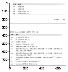
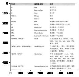
日期的范围、频率以及移动
#将ts转换为一个具有固定频率的时间序列
ts

2011-01-02    0.955968
2011-01-05   -3.053080
2011-01-07   -0.724017
2011-01-08   -1.219987
2011-01-10   -0.303126
2011-01-12   -0.979242
dtype: float64

ts.resample('D')



生成日期范围
index = pd.date_range('4/1/2012','6/1/2012')
index

DatetimeIndex(['2012-04-01', '2012-04-02', '2012-04-03', '2012-04-04',
               '2012-04-05', '2012-04-06', '2012-04-07', '2012-04-08',
               '2012-04-09', '2012-04-10', '2012-04-11', '2012-04-12',
               '2012-04-13', '2012-04-14', '2012-04-15', '2012-04-16',
               '2012-04-17', '2012-04-18', '2012-04-19', '2012-04-20',
               '2012-04-21', '2012-04-22', '2012-04-23', '2012-04-24',
               '2012-04-25', '2012-04-26', '2012-04-27', '2012-04-28',
               '2012-04-29', '2012-04-30', '2012-05-01', '2012-05-02',
               '2012-05-03', '2012-05-04', '2012-05-05', '2012-05-06',
               '2012-05-07', '2012-05-08', '2012-05-09', '2012-05-10',
               '2012-05-11', '2012-05-12', '2012-05-13', '2012-05-14',
               '2012-05-15', '2012-05-16', '2012-05-17', '2012-05-18',
               '2012-05-19', '2012-05-20', '2012-05-21', '2012-05-22',
               '2012-05-23', '2012-05-24', '2012-05-25', '2012-05-26',
               '2012-05-27', '2012-05-28', '2012-05-29', '2012-05-30',
               '2012-05-31', '2012-06-01'],
              dtype='datetime64[ns]', freq='D')

pd.date_range(start='4/1/2012',periods=20)

DatetimeIndex(['2012-04-01', '2012-04-02', '2012-04-03', '2012-04-04',
               '2012-04-05', '2012-04-06', '2012-04-07', '2012-04-08',
               '2012-04-09', '2012-04-10', '2012-04-11', '2012-04-12',
               '2012-04-13', '2012-04-14', '2012-04-15', '2012-04-16',
               '2012-04-17', '2012-04-18', '2012-04-19', '2012-04-20'],
              dtype='datetime64[ns]', freq='D')

pd.date_range(end='6/1/2012',periods=20)

DatetimeIndex(['2012-05-13', '2012-05-14', '2012-05-15', '2012-05-16',
               '2012-05-17', '2012-05-18', '2012-05-19', '2012-05-20',
               '2012-05-21', '2012-05-22', '2012-05-23', '2012-05-24',
               '2012-05-25', '2012-05-26', '2012-05-27', '2012-05-28',
               '2012-05-29', '2012-05-30', '2012-05-31', '2012-06-01'],
              dtype='datetime64[ns]', freq='D')

#生成一个由每月最后一个工作日组成的日期索引，可以传入'BM'频率
pd.date_range('1/1/2000','12/1/2000',freq='BM')

DatetimeIndex(['2000-01-31', '2000-02-29', '2000-03-31', '2000-04-28',
               '2000-05-31', '2000-06-30', '2000-07-31', '2000-08-31',
               '2000-09-29', '2000-10-31', '2000-11-30'],
              dtype='datetime64[ns]', freq='BM')

pd.date_range('5/2/2012 12:56:31',periods=5)

DatetimeIndex(['2012-05-02 12:56:31', '2012-05-03 12:56:31',
               '2012-05-04 12:56:31', '2012-05-05 12:56:31',
               '2012-05-06 12:56:31'],
              dtype='datetime64[ns]', freq='D')

#产生一组被规范化到午夜的时间戳
pd.date_range('5/2/2012 12:56:31',periods=5,normalize=True)

DatetimeIndex(['2012-05-02', '2012-05-03', '2012-05-04', '2012-05-05',
               '2012-05-06'],
              dtype='datetime64[ns]', freq='D')

频率和日期偏移量
from pandas.tseries.offsets import Hour, Minute
hour = Hour()
hour



#传入一个整数既可定义偏移量的倍数
four_hours = Hour(4)
four_hours

<4 * Hours>

pd.date_range('1/1/2000','1/3/2000 23:59',freq='4h')

DatetimeIndex(['2000-01-01 00:00:00', '2000-01-01 04:00:00',
               '2000-01-01 08:00:00', '2000-01-01 12:00:00',
               '2000-01-01 16:00:00', '2000-01-01 20:00:00',
               '2000-01-02 00:00:00', '2000-01-02 04:00:00',
               '2000-01-02 08:00:00', '2000-01-02 12:00:00',
               '2000-01-02 16:00:00', '2000-01-02 20:00:00',
               '2000-01-03 00:00:00', '2000-01-03 04:00:00',
               '2000-01-03 08:00:00', '2000-01-03 12:00:00',
               '2000-01-03 16:00:00', '2000-01-03 20:00:00'],
              dtype='datetime64[ns]', freq='4H')

Hour(2) + Minute(30)

<150 * Minutes>

pd.date_range('1/1/2000',periods=10,freq='1h30min')

DatetimeIndex(['2000-01-01 00:00:00', '2000-01-01 01:30:00',
               '2000-01-01 03:00:00', '2000-01-01 04:30:00',
               '2000-01-01 06:00:00', '2000-01-01 07:30:00',
               '2000-01-01 09:00:00', '2000-01-01 10:30:00',
               '2000-01-01 12:00:00', '2000-01-01 13:30:00'],
              dtype='datetime64[ns]', freq='90T')

#有个知识点
import matplotlib.pyplot as plt
from pylab import *
img = plt.imread('时间序列的基础频率1.png')
imshow(img)


#有个知识点
import matplotlib.pyplot as plt
from pylab import *
img = plt.imread('时间序列的基础频率2.png')
imshow(img)


#每月第三个星期五
rng = pd.date_range('1/1/2012','9/1/2012',freq='WOM-3FRI')
list(rng)

[Timestamp('2012-01-20 00:00:00', freq='WOM-3FRI'),
 Timestamp('2012-02-17 00:00:00', freq='WOM-3FRI'),
 Timestamp('2012-03-16 00:00:00', freq='WOM-3FRI'),
 Timestamp('2012-04-20 00:00:00', freq='WOM-3FRI'),
 Timestamp('2012-05-18 00:00:00', freq='WOM-3FRI'),
 Timestamp('2012-06-15 00:00:00', freq='WOM-3FRI'),
 Timestamp('2012-07-20 00:00:00', freq='WOM-3FRI'),
 Timestamp('2012-08-17 00:00:00', freq='WOM-3FRI')]

移动（超前和滞后）数据
import numpy as np
ts = Series(np.random.randn(4),
           index=pd.date_range('1/1/2000',periods=4,freq='M'))
ts

2000-01-31   -0.085330
2000-02-29    0.111774
2000-03-31    1.852114
2000-04-30   -0.948230
Freq: M, dtype: float64

ts.shift(2)

2000-01-31         NaN
2000-02-29         NaN
2000-03-31   -0.085330
2000-04-30    0.111774
Freq: M, dtype: float64

ts.shift(-2)

2000-01-31    1.852114
2000-02-29   -0.948230
2000-03-31         NaN
2000-04-30         NaN
Freq: M, dtype: float64

ts/ts.shift(1)-1

2000-01-31          NaN
2000-02-29    -2.309908
2000-03-31    15.570148
2000-04-30    -1.511972
Freq: M, dtype: float64

#如果频率已知，还可以实现对时间戳进行位移而不仅仅是对数据进行简单位移
ts.shift(2,freq='M')

2000-03-31   -0.085330
2000-04-30    0.111774
2000-05-31    1.852114
2000-06-30   -0.948230
Freq: M, dtype: float64

ts.shift(3,freq='D')

2000-02-03   -0.085330
2000-03-03    0.111774
2000-04-03    1.852114
2000-05-03   -0.948230
dtype: float64

ts.shift(1,freq='3D')

2000-02-03   -0.085330
2000-03-03    0.111774
2000-04-03    1.852114
2000-05-03   -0.948230
dtype: float64

ts.shift(1,freq='90T')

2000-01-31 01:30:00   -0.085330
2000-02-29 01:30:00    0.111774
2000-03-31 01:30:00    1.852114
2000-04-30 01:30:00   -0.948230
dtype: float64

通过偏移量对日期进行位移
from pandas.tseries.offsets import Day, MonthEnd
now = datetime.datetime(2011,11,17)
now + 3*Day()

Timestamp('2011-11-20 00:00:00')

#加锚点偏移量（如MonthEnd)
now + MonthEnd()

Timestamp('2011-11-30 00:00:00')

now + MonthEnd(2)

Timestamp('2011-12-31 00:00:00')

offset = MonthEnd()
offset.rollforward(now)

Timestamp('2011-11-30 00:00:00')

offset.rollback(now)

Timestamp('2011-10-31 00:00:00')

ts = Series(np.random.randn(20),
           index=pd.date_range('1/15/2000',periods=20,freq='4d'))
ts.groupby(offset.rollforward).mean()

2000-01-31   -0.222426
2000-02-29   -0.607156
2000-03-31   -0.313228
dtype: float64

ts.resample('M').mean()

2000-01-31   -0.222426
2000-02-29   -0.607156
2000-03-31   -0.313228
Freq: M, dtype: float64

时区处理
import pytz
pytz.common_timezones[-5:]

['US/Eastern', 'US/Hawaii', 'US/Mountain', 'US/Pacific', 'UTC']

tz = pytz.timezone('US/Eastern')
tz



本地化和转换
rng = pd.date_range('3/9/2012 9:30',periods=6,freq='D')
ts = Series(np.random.randn(len(rng)),index=rng)
print(ts.index.tz)

None

pd.date_range('3/9/2012 9:30',periods=10,freq='D',tz='UTC')

DatetimeIndex(['2012-03-09 09:30:00+00:00', '2012-03-10 09:30:00+00:00',
               '2012-03-11 09:30:00+00:00', '2012-03-12 09:30:00+00:00',
               '2012-03-13 09:30:00+00:00', '2012-03-14 09:30:00+00:00',
               '2012-03-15 09:30:00+00:00', '2012-03-16 09:30:00+00:00',
               '2012-03-17 09:30:00+00:00', '2012-03-18 09:30:00+00:00'],
              dtype='datetime64[ns, UTC]', freq='D')

#本地化
ts_utc = ts.tz_localize('UTC')
ts_utc

2012-03-09 09:30:00+00:00   -1.562317
2012-03-10 09:30:00+00:00    1.076885
2012-03-11 09:30:00+00:00    0.727747
2012-03-12 09:30:00+00:00    1.327910
2012-03-13 09:30:00+00:00   -0.345919
2012-03-14 09:30:00+00:00   -1.059568
Freq: D, dtype: float64

ts_utc.index

DatetimeIndex(['2012-03-09 09:30:00+00:00', '2012-03-10 09:30:00+00:00',
               '2012-03-11 09:30:00+00:00', '2012-03-12 09:30:00+00:00',
               '2012-03-13 09:30:00+00:00', '2012-03-14 09:30:00+00:00'],
              dtype='datetime64[ns, UTC]', freq='D')

#转换到别的时区
ts_utc.tz_convert('US/Eastern')

2012-03-09 04:30:00-05:00   -1.562317
2012-03-10 04:30:00-05:00    1.076885
2012-03-11 05:30:00-04:00    0.727747
2012-03-12 05:30:00-04:00    1.327910
2012-03-13 05:30:00-04:00   -0.345919
2012-03-14 05:30:00-04:00   -1.059568
Freq: D, dtype: float64

ts_eastern = ts.tz_localize('US/Eastern')
ts_eastern.tz_convert('UTC')

2012-03-09 14:30:00+00:00   -1.562317
2012-03-10 14:30:00+00:00    1.076885
2012-03-11 13:30:00+00:00    0.727747
2012-03-12 13:30:00+00:00    1.327910
2012-03-13 13:30:00+00:00   -0.345919
2012-03-14 13:30:00+00:00   -1.059568
dtype: float64

ts_eastern.tz_convert('Europe/Berlin')

2012-03-09 15:30:00+01:00   -1.562317
2012-03-10 15:30:00+01:00    1.076885
2012-03-11 14:30:00+01:00    0.727747
2012-03-12 14:30:00+01:00    1.327910
2012-03-13 14:30:00+01:00   -0.345919
2012-03-14 14:30:00+01:00   -1.059568
dtype: float64

ts.index.tz_localize('Asia/Shanghai')

DatetimeIndex(['2012-03-09 09:30:00+08:00', '2012-03-10 09:30:00+08:00',
               '2012-03-11 09:30:00+08:00', '2012-03-12 09:30:00+08:00',
               '2012-03-13 09:30:00+08:00', '2012-03-14 09:30:00+08:00'],
              dtype='datetime64[ns, Asia/Shanghai]', freq=None)

操作时区意识型Timestamp对象
stamp = pd.Timestamp('2011-03-12 04:00')
stamp_utc = stamp.tz_localize('utc')
stamp_utc.tz_convert('US/Eastern')

Timestamp('2011-03-11 23:00:00-0500', tz='US/Eastern')

stamp_moscow = pd.Timestamp('2011-03-12 04:00',tz='Europe/Moscow')
stamp_moscow

Timestamp('2011-03-12 04:00:00+0300', tz='Europe/Moscow')

stamp_utc.value

1299902400000000000

stamp_utc.tz_convert('US/Eastern').value

1299902400000000000

#夏令时转变前30分钟
from pandas.tseries.offsets import Hour
stamp = pd.Timestamp('2012-03-12 01:30',tz='US/Eastern')
stamp

Timestamp('2012-03-12 01:30:00-0400', tz='US/Eastern')

stamp + Hour()

Timestamp('2012-03-12 02:30:00-0400', tz='US/Eastern')

#夏令时转变前90分钟
stamp = pd.Timestamp('2012-11-04 00:30',tz='US/Eastern')
stamp

Timestamp('2012-11-04 00:30:00-0400', tz='US/Eastern')

stamp + 2 * Hour()

Timestamp('2012-11-04 01:30:00-0500', tz='US/Eastern')

不同时区之间的运算
rng = pd.date_range('3/7/2012 9:30',periods=10,freq='B')
ts = Series(np.random.randn(len(rng)),index=rng)
ts

2012-03-07 09:30:00    0.610099
2012-03-08 09:30:00   -0.377627
2012-03-09 09:30:00    0.421953
2012-03-12 09:30:00   -0.573061
2012-03-13 09:30:00   -1.092316
2012-03-14 09:30:00   -0.816095
2012-03-15 09:30:00    0.346092
2012-03-16 09:30:00   -0.203076
2012-03-19 09:30:00    0.061797
2012-03-20 09:30:00    0.588646
Freq: B, dtype: float64

ts1 = ts[:7].tz_localize('Europe/London')
ts2 = ts1[2:].tz_convert('Europe/Moscow')
result = ts1+ts2
result.index

DatetimeIndex(['2012-03-07 09:30:00+00:00', '2012-03-08 09:30:00+00:00',
               '2012-03-09 09:30:00+00:00', '2012-03-12 09:30:00+00:00',
               '2012-03-13 09:30:00+00:00', '2012-03-14 09:30:00+00:00',
               '2012-03-15 09:30:00+00:00'],
              dtype='datetime64[ns, UTC]', freq=None)

时期及其算术运算
p = pd.Period(2007,freq='A-DEC')
p

Period('2007', 'A-DEC')

p + 5

Period('2012', 'A-DEC')

p - 2

Period('2005', 'A-DEC')

pd.Period('2014',freq='A-DEC') - p

<7 * YearEnds: month=12>

#创建规则的时期范围
rng = pd.period_range('1/1/2000','6/30/2000',freq='M')
rng

PeriodIndex(['2000-01', '2000-02', '2000-03', '2000-04', '2000-05', '2000-06'], dtype='period[M]')

Series(np.random.randn(6),index=rng)

2000-01   -0.381308
2000-02   -0.433367
2000-03   -1.091356
2000-04    0.276813
2000-05    0.284625
2000-06    0.074151
Freq: M, dtype: float64

values = ['2001Q3','2002Q2','2003Q1']
index = pd.PeriodIndex(values,freq='Q-DEC')
index

PeriodIndex(['2001Q3', '2002Q2', '2003Q1'], dtype='period[Q-DEC]')

时期的频率转换
p = pd.Period('2007',freq='A-DEC')
p.asfreq('M',how='start')

Period('2007-01', 'M')

p.asfreq('M',how='end')

Period('2007-12', 'M')

p = pd.Period('2007',freq='A-JUN')
p.asfreq('M','start')

Period('2006-07', 'M')

p.asfreq('M','end')

Period('2007-06', 'M')

p = pd.Period('2007-08','M')
p.asfreq('A-JUN')

Period('2008', 'A-JUN')

rng = pd.period_range('2006','2009',freq='A-DEC')
ts = Series(np.random.randn(len(rng)),index=rng)
ts

2006    1.185920
2007   -1.529096
2008    1.232203
2009    0.161538
Freq: A-DEC, dtype: float64

ts.asfreq('M',how='start')

2006-01    1.185920
2007-01   -1.529096
2008-01    1.232203
2009-01    0.161538
Freq: M, dtype: float64

ts.asfreq('B',how='end')

2006-12-29    1.185920
2007-12-31   -1.529096
2008-12-31    1.232203
2009-12-31    0.161538
Freq: B, dtype: float64

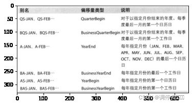
按季度计算的时期频率
p = pd.Period('2012Q4',freq='Q-JAN')
p

Period('2012Q4', 'Q-JAN')

p.asfreq('D','start')

Period('2011-11-01', 'D')

p.asfreq('D','end')

Period('2012-01-31', 'D')

p4pm = (p.asfreq('B','e')-1).asfreq('T','s')+16*60
p4pm

Period('2012-01-30 16:00', 'T')

p4pm.to_timestamp()

Timestamp('2012-01-30 16:00:00')

rng = pd.period_range('2011Q3','2012Q4',freq='Q-JAN')
ts = Series(np.arange(len(rng)),index=rng)
ts

2011Q3    0
2011Q4    1
2012Q1    2
2012Q2    3
2012Q3    4
2012Q4    5
Freq: Q-JAN, dtype: int32

new_rng = (rng.asfreq('B','e')-1).asfreq('T','s')+16*60
ts.index = new_rng.to_timestamp()
ts

2010-10-28 16:00:00    0
2011-01-28 16:00:00    1
2011-04-28 16:00:00    2
2011-07-28 16:00:00    3
2011-10-28 16:00:00    4
2012-01-30 16:00:00    5
dtype: int32

将Timestamp转换为Period（及其反向过程）
rng = pd.date_range('1/1/2000',periods=3,freq='M')
ts = Series(randn(3),index=rng)
pts = ts.to_period()
ts

2000-01-31    0.827634
2000-02-29    0.238047
2000-03-31   -0.154483
Freq: M, dtype: float64

pts

2000-01    0.827634
2000-02    0.238047
2000-03   -0.154483
Freq: M, dtype: float64

rng = pd.date_range('1/29/2000',periods=6,freq='D')
ts2 = Series(randn(6),index=rng)
ts2.to_period('M')

2000-01   -1.799402
2000-01   -0.281554
2000-01   -0.979846
2000-02   -1.499961
2000-02    0.192467
2000-02    0.126386
Freq: M, dtype: float64

pts = ts.to_period()
pts

2000-01    0.827634
2000-02    0.238047
2000-03   -0.154483
Freq: M, dtype: float64

pts.to_timestamp(how='end')

2000-01-31 23:59:59.999999999    0.827634
2000-02-29 23:59:59.999999999    0.238047
2000-03-31 23:59:59.999999999   -0.154483
dtype: float64

通过数组创建PeriodIndex
data = pd.read_csv("E:\python_study_files\python\pydata-book-2nd-edition\examples\macrodata.csv")
data.year

0      1959.0
1      1959.0
2      1959.0
3      1959.0
4      1960.0
        ...  
198    2008.0
199    2008.0
200    2009.0
201    2009.0
202    2009.0
Name: year, Length: 203, dtype: float64

data.quarter

0      1.0
1      2.0
2      3.0
3      4.0
4      1.0
      ... 
198    3.0
199    4.0
200    1.0
201    2.0
202    3.0
Name: quarter, Length: 203, dtype: float64

index = pd.PeriodIndex(year=data.year,quarter=data.quarter,freq='Q-DEC')
index

PeriodIndex(['1959Q1', '1959Q2', '1959Q3', '1959Q4', '1960Q1', '1960Q2',
             '1960Q3', '1960Q4', '1961Q1', '1961Q2',
             ...
             '2007Q2', '2007Q3', '2007Q4', '2008Q1', '2008Q2', '2008Q3',
             '2008Q4', '2009Q1', '2009Q2', '2009Q3'],
            dtype='period[Q-DEC]', length=203)

data.index = index
data.infl

1959Q1    0.00
1959Q2    2.34
1959Q3    2.74
1959Q4    0.27
1960Q1    2.31
          ... 
2008Q3   -3.16
2008Q4   -8.79
2009Q1    0.94
2009Q2    3.37
2009Q3    3.56
Freq: Q-DEC, Name: infl, Length: 203, dtype: float64

重采样及频率转换
将高频率数据聚合到低频率称为降采样，将低频率数据转换到高频率则称为升采样。
rng = pd.date_range('1/1/2000',periods=100,freq='D')
ts = Series(randn(len(rng)),index=rng)
ts.resample('M').mean()

2000-01-31    0.070790
2000-02-29    0.026944
2000-03-31   -0.011548
2000-04-30    0.078033
Freq: M, dtype: float64

ts.resample('M',kind='period').mean()

2000-01    0.070790
2000-02    0.026944
2000-03   -0.011548
2000-04    0.078033
Freq: M, dtype: float64

#有个知识点
import matplotlib.pyplot as plt
from pylab import *
img = plt.imread('resample方法的参数.png')
imshow(img)



[外链图片转存失败,源站可能有防盗链机制,建议将图片保存下来直接上传(img-Amf01oEA-1646554497891)(output_150_1.png)]
降采样
rng = pd.date_range('1/1/2000',periods=12,freq='T')
ts = Series(np.arange(12),index=rng)
ts

2000-01-01 00:00:00     0
2000-01-01 00:01:00     1
2000-01-01 00:02:00     2
2000-01-01 00:03:00     3
2000-01-01 00:04:00     4
2000-01-01 00:05:00     5
2000-01-01 00:06:00     6
2000-01-01 00:07:00     7
2000-01-01 00:08:00     8
2000-01-01 00:09:00     9
2000-01-01 00:10:00    10
2000-01-01 00:11:00    11
Freq: T, dtype: int32

ts.resample('5min').sum()

2000-01-01 00:00:00    10
2000-01-01 00:05:00    35
2000-01-01 00:10:00    21
Freq: 5T, dtype: int32

ts.resample('5min',closed='right').sum()

1999-12-31 23:55:00     0
2000-01-01 00:00:00    15
2000-01-01 00:05:00    40
2000-01-01 00:10:00    11
Freq: 5T, dtype: int32

ts.resample('5min',closed='left',label='left').sum()

2000-01-01 00:00:00    10
2000-01-01 00:05:00    35
2000-01-01 00:10:00    21
Freq: 5T, dtype: int32

ts.resample('5min',loffset='-1s').sum()

C:\windows FutureWarning: 'loffset' in .resample() and in Grouper() is deprecated.

>>> df.resample(freq="3s", loffset="8H")

becomes:

>>> from pandas.tseries.frequencies import to_offset
>>> df = df.resample(freq="3s").mean()
>>> df.index = df.index.to_timestamp() + to_offset("8H")

  ts.resample('5min',loffset='-1s').sum()





1999-12-31 23:59:59    10
2000-01-01 00:04:59    35
2000-01-01 00:09:59    21
Freq: 5T, dtype: int32

OHLC重采样
ts.resample('5min').ohlc()







open
high
low
close




2000-01-01 00:00:00
0
4
0
4


2000-01-01 00:05:00
5
9
5
9


2000-01-01 00:10:00
10
11
10
11



通过groupby进行重采样
rng = pd.date_range('1/1/2000',periods=100,freq='D')
ts = Series(np.arange(100),index=rng)
ts.groupby(lambda x: x.month).mean()

1    15.0
2    45.0
3    75.0
4    95.0
dtype: float64

ts.groupby(lambda x: x.weekday).mean()

0    47.5
1    48.5
2    49.5
3    50.5
4    51.5
5    49.0
6    50.0
dtype: float64

升采样和插值
frame = DataFrame(np.random.randn(2,4),
                 index=pd.date_range('1/1/2000',periods=2,freq='W-WED'),
                 columns=['Colorado','Texas','New York','Ohio'])
frame[:5]







Colorado
Texas
New York
Ohio




2000-01-05
-0.639248
0.966629
1.353138
-0.141245


2000-01-12
-0.202733
2.769799
-0.172722
1.090545



df_daily = frame.resample('D')
df_daily



frame.resample('D').ffill()







Colorado
Texas
New York
Ohio




2000-01-05
-0.639248
0.966629
1.353138
-0.141245


2000-01-06
-0.639248
0.966629
1.353138
-0.141245


2000-01-07
-0.639248
0.966629
1.353138
-0.141245


2000-01-08
-0.639248
0.966629
1.353138
-0.141245


2000-01-09
-0.639248
0.966629
1.353138
-0.141245


2000-01-10
-0.639248
0.966629
1.353138
-0.141245


2000-01-11
-0.639248
0.966629
1.353138
-0.141245


2000-01-12
-0.202733
2.769799
-0.172722
1.090545



frame.resample('D').ffill(limit=2)







Colorado
Texas
New York
Ohio




2000-01-05
-0.639248
0.966629
1.353138
-0.141245


2000-01-06
-0.639248
0.966629
1.353138
-0.141245


2000-01-07
-0.639248
0.966629
1.353138
-0.141245


2000-01-08
NaN
NaN
NaN
NaN


2000-01-09
NaN
NaN
NaN
NaN


2000-01-10
NaN
NaN
NaN
NaN


2000-01-11
NaN
NaN
NaN
NaN


2000-01-12
-0.202733
2.769799
-0.172722
1.090545



frame.resample('W-THU').ffill()







Colorado
Texas
New York
Ohio




2000-01-06
-0.639248
0.966629
1.353138
-0.141245


2000-01-13
-0.202733
2.769799
-0.172722
1.090545



通过时期进行重采样
frame = DataFrame(np.random.randn(24,4),
                 index=pd.period_range('1-2000','12-2001',freq='M'),
                 columns=['Colorado','Texas','New York','Ohio'])
frame[:5]







Colorado
Texas
New York
Ohio




2000-01
-0.111358
-0.647902
-1.546984
-0.723733


2000-02
0.080523
-0.957168
-0.032819
-0.142153


2000-03
-0.357317
0.714370
0.381672
-1.212166


2000-04
-2.072597
-1.275430
-0.972187
0.395826


2000-05
0.204685
0.403605
-0.206892
-0.623941



annual_frame = frame.resample('A-DEC').mean()
annual_frame







Colorado
Texas
New York
Ohio




2000
-0.094581
0.172699
-0.01049
-0.184761


2001
-0.209692
0.172219
-0.16941
-0.244421



#Q-DEC:季度型（每年以12月结束）
annual_frame.resample('Q-DEC').ffill()







Colorado
Texas
New York
Ohio




2000Q1
-0.094581
0.172699
-0.01049
-0.184761


2000Q2
-0.094581
0.172699
-0.01049
-0.184761


2000Q3
-0.094581
0.172699
-0.01049
-0.184761


2000Q4
-0.094581
0.172699
-0.01049
-0.184761


2001Q1
-0.209692
0.172219
-0.16941
-0.244421


2001Q2
-0.209692
0.172219
-0.16941
-0.244421


2001Q3
-0.209692
0.172219
-0.16941
-0.244421


2001Q4
-0.209692
0.172219
-0.16941
-0.244421



annual_frame.resample('Q-DEC',convention='start').ffill()







Colorado
Texas
New York
Ohio




2000Q1
-0.094581
0.172699
-0.01049
-0.184761


2000Q2
-0.094581
0.172699
-0.01049
-0.184761


2000Q3
-0.094581
0.172699
-0.01049
-0.184761


2000Q4
-0.094581
0.172699
-0.01049
-0.184761


2001Q1
-0.209692
0.172219
-0.16941
-0.244421


2001Q2
-0.209692
0.172219
-0.16941
-0.244421


2001Q3
-0.209692
0.172219
-0.16941
-0.244421


2001Q4
-0.209692
0.172219
-0.16941
-0.244421



annual_frame.resample('Q-MAR').ffill()







Colorado
Texas
New York
Ohio




2000Q4
-0.094581
0.172699
-0.01049
-0.184761


2001Q1
-0.094581
0.172699
-0.01049
-0.184761


2001Q2
-0.094581
0.172699
-0.01049
-0.184761


2001Q3
-0.094581
0.172699
-0.01049
-0.184761


2001Q4
-0.209692
0.172219
-0.16941
-0.244421


2002Q1
-0.209692
0.172219
-0.16941
-0.244421


2002Q2
-0.209692
0.172219
-0.16941
-0.244421


2002Q3
-0.209692
0.172219
-0.16941
-0.244421



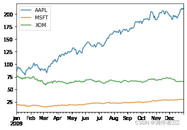
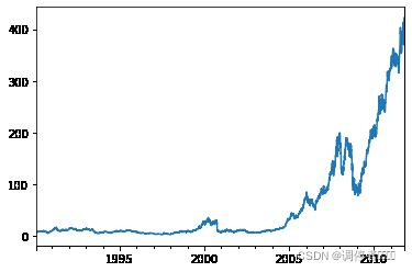
时间序列绘图
close_px_all = pd.read_csv("E:\python_study_files\python\pydata-book-2nd-edition\examples\stock_px.csv",parse_dates=True,index_col=0)
close_px = close_px_all[['AAPL','MSFT','XOM']]
close_px = close_px.resample('B').ffill()
close_px







AAPL
MSFT
XOM




1990-02-01
7.86
0.51
6.12


1990-02-02
8.00
0.51
6.24


1990-02-05
8.18
0.51
6.25


1990-02-06
8.12
0.51
6.23


1990-02-07
7.77
0.51
6.33


...
...
...
...


2011-10-10
388.81
26.94
76.28


2011-10-11
400.29
27.00
76.27


2011-10-12
402.19
26.96
77.16


2011-10-13
408.43
27.18
76.37


2011-10-14
422.00
27.27
78.11



5662 rows × 3 columns
close_px['AAPL'].plot()


close_px.loc['2009'].plot()


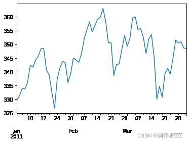
close_px['AAPL'].loc['01-2011':'03-2011'].plot()


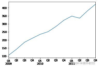
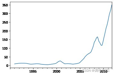
appl_q = close_px['AAPL'].resample('Q-DEC').ffill()
appl_q.loc['2009':].plot()


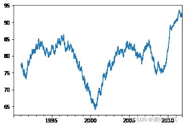
移动窗口函数
close_px.AAPL.plot()


close_px.AAPL.rolling(window=250).mean().plot()


appl_std250 = close_px.AAPL.rolling(window=250,min_periods=10).std()
appl_std250[5:12]

1990-02-08         NaN
1990-02-09         NaN
1990-02-12         NaN
1990-02-13         NaN
1990-02-14    0.148189
1990-02-15    0.141003
1990-02-16    0.135454
Freq: B, Name: AAPL, dtype: float64

appl_std250.plot()


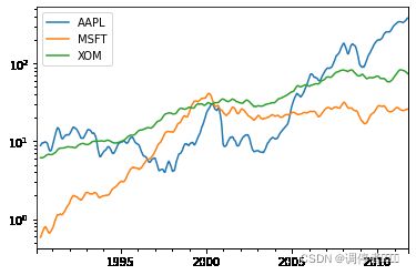
#通过rolling_mean定义扩展平均
expanding_mean = lambda x: x.rolling(window=len(x),min_periods=1).mean()
close_px.rolling(60).mean().plot(logy=True)


#有个知识点
import matplotlib.pyplot as plt
from pylab import *
img = plt.imread('移动窗口和指数加权函数.png')
imshow(img)


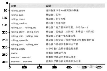
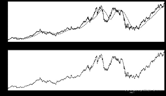
指数加权函数
#指数加权移动平均
fig, axes = plt.subplots(nrows=2,ncols=1,sharex=True,sharey=True,figsize=(12,7))
aapl_px = close_px.AAPL['2005':'2009']
ma60 = aapl_px.rolling(window=60,min_periods=50).mean()
#version 0.18.0之后改成ewm()这个函数了。
ewma60 = pd.DataFrame.ewm(aapl_px,span=60)
aapl_px.plot(style='k-',ax=axes[0])
ma60.plot(style='k--',ax=axes[0])
aapl_px.plot(style='k--',ax=axes[1])
ewma60.plot(style='k--',ax=axes[1])
axes[0].set_title('Simple MA')
axes[1].set_title('Exponentially-weighted MA')

---------------------------------------------------------------------------

AttributeError                            Traceback (most recent call last)

C:\window in 
      8 ma60.plot(style='k--',ax=axes[0])
      9 aapl_px.plot(style='k--',ax=axes[1])
---> 10 ewma60.plot(style='k--',ax=axes[1])
     11 axes[0].set_title('Simple MA')
     12 axes[1].set_title('Exponentially-weighted MA')

AttributeError: 'ExponentialMovingWindow' object has no attribute 'plot'


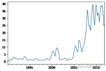
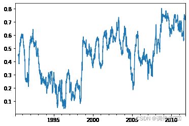
二元移动窗口函数
spx_px = close_px_all['SPX']
spx_rets = spx_px/spx_px.shift(1)-1
returns = close_px.pct_change()
corr = returns.AAPL.rolling(window=125,min_periods=100).corr(spx_rets)
corr.plot()


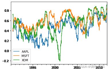
corr = returns.rolling(window=125,min_periods=100).corr(spx_rets)
corr.plot()


用户定义的移动窗口函数
from scipy.stats import percentileofscore
score_at_2percent = lambda x: percentileofscore(x,0.02)
result = returns.AAPL.rolling(window=250).apply(score_at_2percent)
result.plot()


性能和内存使用方面的注意事项
rng = pd.date_range('1/1/2000',periods=10000000,freq='10ms')
ts = Series(np.random.randn(len(rng)),index=rng)
ts

2000-01-01 00:00:00.000   -2.158081
2000-01-01 00:00:00.010   -0.800653
2000-01-01 00:00:00.020   -1.063636
2000-01-01 00:00:00.030   -0.350992
2000-01-01 00:00:00.040    0.025731
                             ...   
2000-01-02 03:46:39.950    1.064119
2000-01-02 03:46:39.960   -1.168419
2000-01-02 03:46:39.970    0.165532
2000-01-02 03:46:39.980   -0.335836
2000-01-02 03:46:39.990    0.906393
Freq: 10L, Length: 10000000, dtype: float64

ts.resample('15min').ohlc()







open
high
low
close




2000-01-01 00:00:00
-2.158081
4.707701
-4.575291
-0.681948


2000-01-01 00:15:00
-1.153593
4.948694
-4.179428
-0.846462


2000-01-01 00:30:00
0.264933
3.978436
-4.369072
-1.591544


2000-01-01 00:45:00
-0.733233
4.702323
-4.718692
-0.031456


2000-01-01 01:00:00
0.409060
4.495952
-4.611355
-0.462664


...
...
...
...
...


2000-01-02 02:45:00
0.543960
4.395054
-4.944563
-0.389855


2000-01-02 03:00:00
-2.653642
3.921464
-4.256564
-0.513813


2000-01-02 03:15:00
-0.429338
4.326163
-4.141456
-0.542056


2000-01-02 03:30:00
-0.739633
4.639564
-4.794910
0.619659


2000-01-02 03:45:00
-0.787038
4.072322
-3.949441
0.906393



112 rows × 4 columns
%timeit ts.resample('15min').ohlc()

109 ms ± 3.1 ms per loop (mean ± std. dev. of 7 runs, 10 loops each)

%timeit ts.resample('15s').ohlc()

113 ms ± 2.48 ms per loop (mean ± std. dev. of 7 runs, 10 loops each)

	Colorado	Texas	New York	Ohio
2001-05-02	-1.864282	0.085645	-1.803818	0.923839
2001-05-09	0.344391	0.471942	2.089121	-1.123721
2001-05-16	0.770508	0.618750	-0.787188	-1.083100
2001-05-23	0.743285	-0.468671	0.610547	0.957291
2001-05-30	0.343177	-1.018066	1.196951	-0.434751

	open	high	low	close
2000-01-01 00:00:00	0	4	0	4
2000-01-01 00:05:00	5	9	5	9
2000-01-01 00:10:00	10	11	10	11

	Colorado	Texas	New York	Ohio
2000-01-05	-0.639248	0.966629	1.353138	-0.141245
2000-01-12	-0.202733	2.769799	-0.172722	1.090545

	Colorado	Texas	New York	Ohio
2000-01-05	-0.639248	0.966629	1.353138	-0.141245
2000-01-06	-0.639248	0.966629	1.353138	-0.141245
2000-01-07	-0.639248	0.966629	1.353138	-0.141245
2000-01-08	-0.639248	0.966629	1.353138	-0.141245
2000-01-09	-0.639248	0.966629	1.353138	-0.141245
2000-01-10	-0.639248	0.966629	1.353138	-0.141245
2000-01-11	-0.639248	0.966629	1.353138	-0.141245
2000-01-12	-0.202733	2.769799	-0.172722	1.090545

	Colorado	Texas	New York	Ohio
2000-01-05	-0.639248	0.966629	1.353138	-0.141245
2000-01-06	-0.639248	0.966629	1.353138	-0.141245
2000-01-07	-0.639248	0.966629	1.353138	-0.141245
2000-01-08	NaN	NaN	NaN	NaN
2000-01-09	NaN	NaN	NaN	NaN
2000-01-10	NaN	NaN	NaN	NaN
2000-01-11	NaN	NaN	NaN	NaN
2000-01-12	-0.202733	2.769799	-0.172722	1.090545

	Colorado	Texas	New York	Ohio
2000-01-06	-0.639248	0.966629	1.353138	-0.141245
2000-01-13	-0.202733	2.769799	-0.172722	1.090545

	Colorado	Texas	New York	Ohio
2000-01	-0.111358	-0.647902	-1.546984	-0.723733
2000-02	0.080523	-0.957168	-0.032819	-0.142153
2000-03	-0.357317	0.714370	0.381672	-1.212166
2000-04	-2.072597	-1.275430	-0.972187	0.395826
2000-05	0.204685	0.403605	-0.206892	-0.623941

	Colorado	Texas	New York	Ohio
2000	-0.094581	0.172699	-0.01049	-0.184761
2001	-0.209692	0.172219	-0.16941	-0.244421

	Colorado	Texas	New York	Ohio
2000Q1	-0.094581	0.172699	-0.01049	-0.184761
2000Q2	-0.094581	0.172699	-0.01049	-0.184761
2000Q3	-0.094581	0.172699	-0.01049	-0.184761
2000Q4	-0.094581	0.172699	-0.01049	-0.184761
2001Q1	-0.209692	0.172219	-0.16941	-0.244421
2001Q2	-0.209692	0.172219	-0.16941	-0.244421
2001Q3	-0.209692	0.172219	-0.16941	-0.244421
2001Q4	-0.209692	0.172219	-0.16941	-0.244421

	Colorado	Texas	New York	Ohio
2000Q1	-0.094581	0.172699	-0.01049	-0.184761
2000Q2	-0.094581	0.172699	-0.01049	-0.184761
2000Q3	-0.094581	0.172699	-0.01049	-0.184761
2000Q4	-0.094581	0.172699	-0.01049	-0.184761
2001Q1	-0.209692	0.172219	-0.16941	-0.244421
2001Q2	-0.209692	0.172219	-0.16941	-0.244421
2001Q3	-0.209692	0.172219	-0.16941	-0.244421
2001Q4	-0.209692	0.172219	-0.16941	-0.244421

	Colorado	Texas	New York	Ohio
2000Q4	-0.094581	0.172699	-0.01049	-0.184761
2001Q1	-0.094581	0.172699	-0.01049	-0.184761
2001Q2	-0.094581	0.172699	-0.01049	-0.184761
2001Q3	-0.094581	0.172699	-0.01049	-0.184761
2001Q4	-0.209692	0.172219	-0.16941	-0.244421
2002Q1	-0.209692	0.172219	-0.16941	-0.244421
2002Q2	-0.209692	0.172219	-0.16941	-0.244421
2002Q3	-0.209692	0.172219	-0.16941	-0.244421

	AAPL	MSFT	XOM
1990-02-01	7.86	0.51	6.12
1990-02-02	8.00	0.51	6.24
1990-02-05	8.18	0.51	6.25
1990-02-06	8.12	0.51	6.23
1990-02-07	7.77	0.51	6.33
...	...	...	...
2011-10-10	388.81	26.94	76.28
2011-10-11	400.29	27.00	76.27
2011-10-12	402.19	26.96	77.16
2011-10-13	408.43	27.18	76.37
2011-10-14	422.00	27.27	78.11

	open	high	low	close
2000-01-01 00:00:00	-2.158081	4.707701	-4.575291	-0.681948
2000-01-01 00:15:00	-1.153593	4.948694	-4.179428	-0.846462
2000-01-01 00:30:00	0.264933	3.978436	-4.369072	-1.591544
2000-01-01 00:45:00	-0.733233	4.702323	-4.718692	-0.031456
2000-01-01 01:00:00	0.409060	4.495952	-4.611355	-0.462664
...	...	...	...	...
2000-01-02 02:45:00	0.543960	4.395054	-4.944563	-0.389855
2000-01-02 03:00:00	-2.653642	3.921464	-4.256564	-0.513813
2000-01-02 03:15:00	-0.429338	4.326163	-4.141456	-0.542056
2000-01-02 03:30:00	-0.739633	4.639564	-4.794910	0.619659
2000-01-02 03:45:00	-0.787038	4.072322	-3.949441	0.906393

【Python】一文详细介绍 py格式文件高斯小哥 Python基础【高质量合集】python 新手入门学习
【Python】一文详细介绍py格式文件个人主页：高斯小哥高质量专栏：Matplotlib之旅：零基础精通数据可视化、Python基础【高质量合集】、PyTorch零基础入门教程希望得到您的订阅和支持~创作高质量博文(平均质量分92+)，分享更多关于深度学习、PyTorch、Python领域的优质内容！（希望得到您的关注~）文章目录一、py格式文件简介二、如何创建和编辑py格式文件三、如何运行py
python抓包与解包_Python—网络抓包与解包（pcap、dpkt） weixin_39691055 python抓包与解包
pcap安装[root@localhost~]#pipinstallpypcap抓包与解包#-*-coding:utf-8-*-importpcap,dpktimportre,threading,requests__black_ip=['103.224.249.123','203.66.1.212']#抓包：param1eth_name网卡名，如：eth0,eth3。param2p_type日志捕
新网师的精神肤色（幕布笔记）悦读书香
王子老师的《极简100小妙招》收到已经几天了，之前大概的浏览了全书，今天起给自己定了一个计划，必须每天学习极简小妙招里面的一个妙招，并加以运用。一、今天要打卡什么内容因有完成每天学习极简小妙招的计划，所以今天晚饭吃的比较简单，草草吃完以后带着小宝到广场溜达一圈，急忙赶回来学习极简小妙招。再重看的时候不知道自己要学点什么，打卡哪一招，感觉哪个都简单，就看这一环节像王子老师说的“一看就会”，但做这一环
华为OD机试 - 单向链表中间节点（Java & JS & Python & C & C++）华为OD题库华为od 链表 java
须知哈喽，本题库完全免费，收费是为了防止被爬，大家订阅专栏后可以私信联系退款。感谢支持文章目录须知题目描述输出描述解析代码题目描述给定一个单链表L，请编写程序输出L中间结点保存的数据。如果有两个中间结点，则输出第二个中间结点保存的数据。例如：给定L为1→7→5，则输出应该为7；给定L为1→2→3→4，则输出应该为3；输入描述每个输入包含1个测试用例。每个测试用例：第一行给出链表首结点的地址、结点总
python 推导式(派生、衍生) sanduo112 人工智能 python windows 开发语言
python推导式一、推导式(派生、衍生)1.Python推导式是一种独特的数据处理方式，可以从一个数据序列构建另一个新的数据序列的结构体。2.列表(list)推导式3.字典(dict)推导式4.集合(set)推导式5.元组(tuple)推导式二、代码概述一、推导式(派生、衍生)1.Python推导式是一种独特的数据处理方式，可以从一个数据序列构建另一个新的数据序列的结构体。Python支持各种数
数据挖掘|数据预处理|基于Python的数据标准化方法皖山文武数据挖掘数据建模与分析 python 数据挖掘开发语言
基于Python的数据标准化方法1.z-score方法2.极差标准化方法3.最大绝对值标准化方法在数据分析之前，通常需要先将数据标准化（Standardization），利用标准化后的数据进行数据分析，以避免属性之间不同度量和取值范围差异造成数据对分析结果的影响。1.z-score方法Z-score方法是基于原始数据的均值和标准差来进行数据标准化的，处理后的数据均值为0，方差为1，符合标准正态分布
C++学习笔记（lambda函数） __TAT__ C&C++c++学习笔记
C++learningnote1、lambda函数的语法2、lambda函数的几种用法1、lambda函数的语法lambda函数的一般语法如下：[capture_clause](parameters)->return_type{function_body}capture_clause：需要捕获的变量，但要求该变量必须在这个作用域中。通常的捕获方式有以下几种：[]：不捕获任何变量[&]：按引用捕获变
CSV指南：Python程序获取大型CSV文件行数孤独打铁匠Julian 笔记经验分享 python
本指南提供了几种使用Python来获取大型CSV文件行数的方法，并解释了每种方法的适用场景。方法1:使用csv.reader处理复杂CSV文件当你的CSV文件中包含多行字段（即某些字段的值中包含换行符）时，使用csv.reader是一个可靠的选择，因为它能够正确处理这些复杂情况。这个方法适用于大多数大小的CSV文件，但是对于非常大的文件，读取整个文件可能会占用较多的时间和内存。对于极大的文件，考虑
谷歌浏览器驱动Chromedriver（114-120版本）文件以及驱动下载教程 pigerr杨 Python python chrome drivers
ChromeDriver官方网站GitHub||GoogleChromeLabs/chrome-for-testingChromeDriver113-125_JSONChromeforTestingavailability123-125zip白月黑羽Python基础|进阶|Qt图形界面|Django|自动化测试|性能测试|JS语言|JS前端|原理与安装
大创项目推荐深度学习 opencv python 公式识别(图像识别机器视觉) laafeer python
文章目录0前言1课题说明2效果展示3具体实现4关键代码实现5算法综合效果6最后0前言优质竞赛项目系列，今天要分享的是基于深度学习的数学公式识别算法实现该项目较为新颖，适合作为竞赛课题方向，学长非常推荐！学长这里给一个题目综合评分(每项满分5分)难度系数：3分工作量：4分创新点：4分更多资料,项目分享：https://gitee.com/dancheng-senior/postgraduate1课题
读书笔记《穿越寒冬》如雪般飞舞
各位好，我们今天来讲一本书，名字叫作《穿越寒冬》。看起来特别应景，大家觉得现在创业的状况不景气，大家都在忍受着寒冬的煎熬。但实际上，这本书的英文名字并不是这个意思，它的英文名叫作“如何创立一家新公司，并且能够活下来”。我在整个读完了以后，我发现这本书真正要翻译得好，它的名字应该叫作《创业生存手册》。这个书的作者，来自硅谷的霍夫曼船长。霍夫曼船长写过一本让创业者觉得特别贴心的书，叫作《让大象飞》它和
2018-11-18成长小组学习笔记实验中学45
因为嗓子“罢工”，我面对众人只能借“微笑”代言。在开始授课前，绣霞老师先反馈上次作业的情况，提到“接纳”需是真正发自内心的完全接纳，而不是口头上的接纳，内心却是排斥的。提到一个“问题”孩子恰恰对家爱的更加“深沉”，夫妻间的问题不能影响到孩子，对孩子更好的爱不是你为他做的更多，而是给他自由、健康成长的空间。图片发自App一、孩子：家庭的一面镜子夫妻成了彼此的“投射”，婚姻便“吵的不可开交”，婚姻便成
【鸿蒙HarmonyOS开发笔记】ArkUI常用组件介绍汇总（更新中）温、鸿蒙HarmonyOS开发笔记学习记录 harmonyos 笔记华为
概述此文总结开发中用到的一些常用组件，便于查阅，此文持续更新，闲的没事就更线性布局（Row/Column）不多介绍了，最常用的布局组件，两者除了方向不一样，别的都一样方便起见下面只写Column常用属性排列方向上的间距：spaceColumn({space:20}){Row().width('90%').height(50).backgroundColor(0xF5DEB3)Row().width
python转码 Desamond python 开发语言
转码在许多场景中都有应用，以下是一些常见的场景：网页开发：当用户在网页上输入文本时，可能需要将特殊字符（如空格、引号、特殊符号等）进行转码，以防止这些字符对URL或HTML代码产生干扰。文件名处理：在处理文件名时，可能需要将特殊字符进行转码，以避免文件名被错误地解析或显示。数据传输：在数据传输过程中，为了确保数据的完整性和正确性，可能需要将数据中的特殊字符进行转码。数据存储：在数据库或数据存储中，
排序算法太多？常用排序都在这了，一篇文章总结和实现所有面试会考的排序算法（基于Python实现）宇宙之一粟不归路之Python #IT面试题收集与总结数据结构与算法算法数据结构排序算法 python java
文章目录排序算法1.常见的排序算法1.1选择排序1.1.1思想1.1.2实现**1.1.3选择排序分析**1.2冒泡排序**1.2.1思想****1.2.2实现****1.2.3冒泡排序分析**1.3插入排序**1.3.1思想****1.3.2实现****1.3.3插入排序分析**1.4归并排序☆☆★**1.4.1思想****1.4.2实现****1.4.3归并排序分析**1.5快速排序☆★★**
27.Python从入门到精通—Python异常处理抛出异常用户自定义异常定义清理行为预定义的清理行为以山河作礼。 #Python基础入门—详解版 python java 服务器
27.从入门到精通：Python异常处理抛出异常用户自定义异常定义清理行为预定义的清理行为异常处理抛出异常用户自定义异常定义清理行为预定义的清理行为异常处理在Python中，异常处理是一种处理程序在执行期间可能遇到的错误的方法。当Python解释器遇到错误时，它会引发异常。异常是一种Python对象，它包含有关错误的信息，例如错误类型和错误位置。为了处理异常，您可以使用try-except语句。在
python清华大学出版社答案_Python机器学习及实践 weixin_39805119 python清华大学出版社答案
第1章机器学习的基础知识1.1何谓机器学习1.1.1传感器和海量数据1.1.2机器学习的重要性1.1.3机器学习的表现1.1.4机器学习的主要任务1.1.5选择合适的算法1.1.6机器学习程序的步骤1.2综合分类1.3推荐系统和深度学习1.3.1推荐系统1.3.2深度学习1.4何为Python1.4.1使用Python软件的由来1.4.2为什么使用Python1.4.3Python设计定位1.4.
安卓笔记本 - Handler Message MessageQueue Looper SocialException
不爱写字，一张图解决。Handler,Message,MessageQueue,Looper工作原理
枚举使用笔记万变不离其宗_8 项目笔记笔记
1.java枚举怎么放在方法上面的注释里面/***保存*@paramuserId用户id*@paramtype见枚举{@linkcom.common.enums.TypeEnum}*@return*/voidsave(LonguserId,Stringtype);
ruoyi使用笔记万变不离其宗_8 项目笔记代码参考笔记笔记 java 前端
1.限流处理@RateLimiter@PostMapping("/createOrder")@ApiOperation("创建充值订单")@RateLimiter(key=CacheConstants.REPEAT_SUBMIT_KEY,time=10,count=1,limitType=LimitType.IP)publicRcreateOrder(@RequestBodyFormform){/
Python | Redis工具类 -拟墨画扇- Python redis 数据库缓存 python
一、需求自动连接Redis数据库，通过连接池处理数据对输出结果进行Log打印并保存到文件二、代码Utils.redisUtils.py#!/usr/bin/envpython#-*-coding:utf-8-*-importredisfromUtils.loggerimportlog"""Redis数据格式(1)字符串|存储形式:key-value:str-存储二进制数据:可以存储任意类型的数据，
数据管理知识体系指南（第二版）-第五章——数据建模和设计-学习笔记键盘上的五花肉数据治理数据库数据仓库数据治理
目录5.1引言5.1.1业务驱动因素5.1.2目标和原则5.1.3基本概念5.2活动5.2.1规划数据建模5.2.2建立数据模型5.2.3审核数据模型5.2.4维护数据模型5.3工具5.3.1数据建模工具5.3.2数据血缘工具5.3.3数据分析工具5.3.4元数据资料库5.3.5数据模型模式5.3.6行业数据模型5.4方法5.4.1命名约定的最佳实践5.4.2数据库设计中的最佳实践5.5数据建模和
Python dict字符串转json对象，小数精度丢失问题朝如青丝暮成雪 json python
一前言JSON(JavaScriptObjectNotation)是一种轻量级的数据交换格式，dict是Python的一种数据格式。本篇介绍一个float数据转换时精度丢失的案例。二问题描述importjsontest_str1='{"π":3.1415926535897932384626433832795028841971}'test_str2='{"value":10.00000}'print
java实体中返回前端的double类型四舍五入（格式化）婲落ヽ紅顏誶 java
根据业务，需要通过后端给前端返回部分double类型的数值，一般需要保留两位小数，使用jackson转换对象packagecom.ruoyi.common.core.config;importcom.fasterxml.jackson.core.JsonGenerator;importcom.fasterxml.jackson.databind.JsonSerializer;importcom.f
Django forms组件在飞行-米龙 Django django python 后端
【一】引入【1】实现登陆验证功能（1）需求分析登陆验证需要前后端交互，采用form表单提交数据对数据进行校验用户名必须以英文大写字母开头密码必须大于三位数反馈给用户错误的信息除了反馈错误的信息还有保留原始输入内容（2）后端代码使用user_info_dict字典每次刷新存储存储前端发送的信息存储后端进行验证的信息defhome(request):#每次后刷新这个信息字典user_info_dict
Java学习笔记01 .wsy. 日常 java 学习笔记
1.1Java简介Java的前身是Oak，詹姆斯·高斯林是java之父。1.2Java体系Java是一种与平台无关的语言，其源代码可以被编译成一种结构中立的中间文件（.class，字节码文件）于Java虚拟机上运行。1.2.3专有名词JDK提供编译、运行Java程序所需要的种种工具及资源。JRE是运行Java所依赖的环境的集合。JVM是一个虚构出来的计算机，通过在实际的计算机上仿真模拟各种计算机功
Webpack构建优化——区分环境 oWSQo
为什么需要区分环境在开发网页的时候，一般都会有多套运行环境，例如：在开发过程中方便开发调试的环境。发布到线上给用户使用的运行环境。这两套不同的环境虽然都是由同一套源代码编译而来，但是代码内容却不一样，差异包括：线上代码被特殊压缩过。开发用的代码包含一些用于提示开发者的提示日志，这些日志普通用户不可能去看它。开发用的代码所连接的后端数据接口地址也可能和线上环境不同，因为要避免开发过程中造成对线上数据
Python+Requests模拟发送GET请求爱学习的执念自动化测试软件测试技术分享 python 开发语言
模拟发送GET请求前置条件：导入requests库一、发送不带参数的get请求代码如下：以百度首页为例importrequests#发送get请求response=requests.get(url="http://www.baidu.com")print(response.content.decode("utf-8"))#以utf-8的编码输出内容二、发送带参数的get请求发送带参数的get请求有
《老子》笔记19 2018-10-28 海上明月共
第二十二章[原文]曲则全，枉则直，洼则盈，敝则新，少则得，多则惑。是以圣人抱一为天下式。不自见，故明；不自是，故彰，不自伐，故有功；不自矜，故长。夫唯不争，故天下莫能与之争。古之所谓"曲则全"者，岂虚言哉？诚全而归之。[译文]委曲便会保全，屈枉便会直伸；低洼便会充盈，陈旧便会更新；少取便会获得，贪多便会迷惑。所以有道的人坚守这一原则作为天下事理的范式，不自我表扬，反能显明；不自以为是，反能是非彰明
Python极速入门：五分钟开启实战之旅！知白守黑V Python 编程语言系统运维 python 编程语言 python开发 python学习 python入门 python数据分析
1.Python基础语法和结构：了解Python的基本语法，包括变量、数据类型、运算符、注释等。控制流：掌握条件语句（if-elif-else）、循环（for和while）及其控制（break和continue）。函数：学习如何定义和使用函数，包括参数传递、返回值、作用域和闭包。模块和包：理解如何导入和使用模块，以及如何创建和使用自己的包。2.数据处理列表、元组和集合：学习这些序列类型的操作和方法
C/C++Win32编程基础详解视频下载择善Zach 编程 C++Win32
课题视频：C/C++Win32编程基础详解视频知识：win32窗口的创建 windows事件机制主讲：择善Uncle老师学习交流群：386620625 验证码：625 --
Guava Cache使用笔记 bylijinnan java guava cache
1.Guava Cache的get/getIfPresent方法当参数为null时会抛空指针异常我刚开始使用时还以为Guava Cache跟HashMap一样，get(null)返回null。实际上Guava整体设计思想就是拒绝null的，很多地方都会执行com.google.common.base.Preconditions.checkNotNull的检查。 2.Guava
解决ora-01652无法通过128（在temp表空间中） 0624chenhong oracle
解决ora-01652无法通过128（在temp表空间中）扩展temp段的过程一个sql语句后，大约花了10分钟，好不容易有一个结果，但是报了一个ora-01652错误，查阅了oracle的错误代码说明：意思是指temp表空间无法自动扩展temp段。这种问题一般有两种原因：一是临时表空间空间太小，二是不能自动扩展。分析过程：既然是temp表空间有问题，那当
Struct在jsp标签不懂事的小屁孩 struct
非UI标签介绍：控制类标签： 1：程序流程控制标签 if elseif else <s:if test="isUsed"> <span class="label label-success">True</span> </
按对象属性排序换个号韩国红果果 JavaScript 对象排序
利用JavaScript进行对象排序，根据用户的年龄排序展示 <script> var bob={ name;bob, age:30 } var peter={ name;peter, age:30 } var amy={ name;amy, age:24 } var mike={ name;mike, age:29 } var john={
大数据分析让个性化的客户体验不再遥远蓝儿唯美数据分析
顾客通过多种渠道制造大量数据，企业则热衷于利用这些信息来实现更为个性化的体验。分析公司Gartner表示，高级分析会成为客户服务的关键，但是大数据分析的采用目前仅局限于不到一成的企业。挑战在于企业还在努力适应结构化数据，疲于根据自身的客户关系管理（CRM）系统部署有效的分析框架，以及集成不同的内外部信息源。然而，面对顾客通过数字技术参与而产生的快速变化的信息，企业需要及时作出反应。要想实
java笔记4 a-john java
操作符 1，使用java操作符操作符接受一个或多个参数，并生成一个新值。参数的形式与普通的方法调用不用，但是效果是相同的。加号和一元的正号（+）、减号和一元的负号（-）、乘号（*）、除号（/）以及赋值号（=）的用法与其他编程语言类似。操作符作用于操作数，生成一个新值。另外，有些操作符可能会改变操作数自身的
从裸机编程到嵌入式Linux编程思想的转变------分而治之：驱动和应用程序 aijuans 嵌入式学习
笔者学习嵌入式Linux也有一段时间了，很奇怪的是很多书讲驱动编程方面的知识，也有很多书将ARM9方面的知识，但是从以前51形式的（对寄存器直接操作，初始化芯片的功能模块）编程方法，和思维模式，变换为基于Linux操作系统编程，讲这个思想转变的书几乎没有，让初学者走了很多弯路，撞了很多难墙。笔者因此写上自己的学习心得，希望能给和我一样转变
在springmvc中解决FastJson循环引用的问题 asialee 循环引用 fastjson
我们先来看一个例子： package com.elong.bms; import java.io.OutputStream; import java.util.HashMap; import java.util.Map; import co
ArrayAdapter和SimpleAdapter技术总结百合不是茶 android SimpleAdapter ArrayAdapter 高级组件基础
ArrayAdapter比较简单，但它只能用于显示文字。而SimpleAdapter则有很强的扩展性，可以自定义出各种效果 ArrayAdapter;的数据可以是数组或者是队列 // 获得下拉框对象 AutoCompleteTextView textview = (AutoCompleteTextView) this
九封信 bijian1013 人生励志
有时候，莫名的心情不好，不想和任何人说话，只想一个人静静的发呆。有时候，想一个人躲起来脆弱，不愿别人看到自己的伤口。有时候，走过熟悉的街角，看到熟悉的背影，突然想起一个人的脸。有时候，发现自己一夜之间就长大了。 2014，写给人
Linux下安装MySQL Web 管理工具phpMyAdmin sunjing PHP Install phpMyAdmin
PHP http://php.net/ phpMyAdmin http://www.phpmyadmin.net Error compiling PHP on CentOS x64 一、安装Apache 请参阅http://billben.iteye.com/admin/blogs/1985244 二、安装依赖包 sudo yum install gd
分布式系统理论 bit1129 分布式
FLP One famous theory in distributed computing, known as FLP after the authors Fischer, Lynch, and Patterson, proved that in a distributed system with asynchronous communication and process crashes,
ssh2整合(spring+struts2+hibernate)-附源码白糖_ eclipse spring Hibernate mysql 项目管理
最近抽空又整理了一套ssh2框架，主要使用的技术如下： spring做容器，管理了三层(dao,service,actioin)的对象 struts2实现与页面交互(MVC)，自己做了一个异常拦截器，能拦截Action层抛出的异常 hibernate与数据库交互 BoneCp数据库连接池，据说比其它数据库连接池快20倍，仅仅是据说 MySql数据库项目用eclipse
treetable bug记录 braveCS table
// 插入子节点删除再插入时不能正常显示。修改： //不知改后有没有错，先做个备忘 Tree.prototype.removeNode = function(node) { // Recursively remove all descendants of +node+ this.unloadBranch(node); // Remove
编程之美-电话号码对应英语单词 bylijinnan java 算法编程之美
import java.util.Arrays; public class NumberToWord { /** * 编程之美电话号码对应英语单词 * 题目： * 手机上的拨号盘，每个数字都对应一些字母，比如2对应ABC，3对应DEF.........，8对应TUV，9对应WXYZ， * 要求对一段数字，输出其代表的所有可能的字母组合
jquery ajax读书笔记 chengxuyuancsdn jQuery ajax
1、jsp页面 <%@ page language="java" import="java.util.*" pageEncoding="GBK"%> <% String path = request.getContextPath(); String basePath = request.getScheme()
JWFD工作流拓扑结构解析伪码描述算法 comsci 数据结构算法工作活动 J#
对工作流拓扑结构解析感兴趣的朋友可以下载附件，或者下载JWFD的全部代码进行分析 /* 流程图拓扑结构解析伪码描述算法 public java.util.ArrayList DFS(String graphid, String stepid, int j)
oracle I/O 从属进程 daizj oracle
I/O 从属进程　　I/O从属进程用于为不支持异步I/O的系统或设备模拟异步I/O.例如，磁带设备(相当慢)就不支持异步I/O.通过使用I/O 从属进程，可以让磁带机模仿通常只为磁盘驱动器提供的功能。就好像支持真正的异步I/O 一样，写设备的进程(调用者)会收集大量数据，并交由写入器写出。数据成功地写出时，写入器(此时写入器是I/O 从属进程，而不是操作系统)会通知原来的调用者，调用者则会
高级排序:希尔排序 dieslrae 希尔排序
public void shellSort(int[] array){ int limit = 1; int temp; int index; while(limit <= array.length/3){ limit = limit * 3 + 1;
初二下学期难记忆单词 dcj3sjt126com english word
kitchen 厨房 cupboard 厨柜 salt 盐 sugar 糖 oil 油 fork 叉；餐叉 spoon 匙；调羹 chopsticks 筷子 cabbage 卷心菜；洋白菜 soup 汤 Italian 意大利的 Indian 印度的 workplace 工作场所 even 甚至；更 Italy 意大利 laugh 笑 m
Go语言使用MySQL数据库进行增删改查 dcj3sjt126com mysql
目前Internet上流行的网站构架方式是LAMP，其中的M即MySQL, 作为数据库，MySQL以免费、开源、使用方便为优势成为了很多Web开发的后端数据库存储引擎。MySQL驱动Go中支持MySQL的驱动目前比较多，有如下几种，有些是支持database/sql标准，而有些是采用了自己的实现接口,常用的有如下几种: http://code.google.c...o-mysql-dri
git命令 shuizhaosi888 git
---------------设置全局用户名： git config --global user.name "HanShuliang" //设置用户名 git config --global user.email "[email protected]" //设置邮箱 ---------------查看环境配置 git config --li
qemu-kvm 网络 nat模式 (四) haoningabc kvm qemu
qemu-ifup-NAT #!/bin/bash BRIDGE=virbr0 NETWORK=192.168.122.0 GATEWAY=192.168.122.1 NETMASK=255.255.255.0 DHCPRANGE=192.168.122.2,192.168.122.254 TFTPROOT= BOOTP= function check_bridge()
不要让未来的你，讨厌现在的自己 jingjing0907 生活奋斗工作梦想
故事one 　23岁，他大学毕业，放弃了父母安排的稳定工作，独闯京城，在家小公司混个小职位，工作还算顺手，月薪三千，混了混，混走了一年的光阴。　　　　24岁，有了女朋友，从二环12人的集体宿舍搬到香山民居，一间平房，二人世界，爱爱爱。偶然约三朋四友，打扑克搓麻将，日子快乐似神仙；　　　　25岁，出了几次差，调了两次岗，薪水涨了不过百，生猛狂飙的物价让现实血淋淋，无力为心爱银儿购件大牌
枚举类型详解一路欢笑一路走 enum 枚举详解 enumset enumMap
枚举类型详解一.Enum详解 1.1枚举类型的介绍 JDK1.5加入了一个全新的类型的”类”—枚举类型，为此JDK1.5引入了一个新的关键字enum,我们可以这样定义一个枚举类型。 Demo:一个最简单的枚举类 public enum ColorType { RED
第11章动画效果（上） onestopweb 动画
index.html <!DOCTYPE html PUBLIC "-//W3C//DTD XHTML 1.0 Transitional//EN" "http://www.w3.org/TR/xhtml1/DTD/xhtml1-transitional.dtd"> <html xmlns="http://www.w3.org/
Eclipse中jsp、js文件编辑时，卡死现象解决汇总 ljf_home eclipse jsp卡死 js卡死
使用Eclipse编辑jsp、js文件时，经常出现卡死现象，在网上百度了N次，经过N次优化调整后，卡死现象逐步好转，具体那个方法起到作用，不太好讲。将所有用过的方法罗列如下： 1、取消验证 windows–>perferences–>validation 把除了manual 下面的全部点掉，build下只留 classpath dependency Valida
MySQL编程中的6个重要的实用技巧 tomcat_oracle mysql
每一行命令都是用分号(;)作为结束对于MySQL，第一件你必须牢记的是它的每一行命令都是用分号(;)作为结束的，但当一行MySQL被插入在PHP代码中时，最好把后面的分号省略掉，例如： mysql_query("INSERT INTO tablename(first_name,last_name)VALUES('$first_name',$last_name')");
zoj 3820 Building Fire Stations(二分+bfs) 阿尔萨斯 Build
题目链接：zoj 3820 Building Fire Stations 题目大意：给定一棵树，选取两个建立加油站，问说所有点距离加油站距离的最大值的最小值是多少，并且任意输出一种建立加油站的方式。解题思路：二分距离判断，判断函数的复杂度是o(n)，这样的复杂度应该是o(nlogn)，即使常数系数偏大，但是居然跑了4.5s，也是醉了。判断函数里面做了3次bfs，但是每次bfs节点最多

利用Python进行数据分析的学习笔记——chap10

时间序列

日期和时间数据类型及工具

字符串和datetime的相互转换

时间序列基础

索引、选取、子集构造

带有重复索引的时间序列

日期的范围、频率以及移动

生成日期范围

频率和日期偏移量

移动（超前和滞后）数据

通过偏移量对日期进行位移

时区处理

本地化和转换

操作时区意识型Timestamp对象

不同时区之间的运算

时期及其算术运算

时期的频率转换

按季度计算的时期频率

将Timestamp转换为Period（及其反向过程）

通过数组创建PeriodIndex

重采样及频率转换

降采样

OHLC重采样

通过groupby进行重采样

升采样和插值

通过时期进行重采样

时间序列绘图

移动窗口函数

指数加权函数

二元移动窗口函数

用户定义的移动窗口函数

性能和内存使用方面的注意事项

你可能感兴趣的:(笔记,python,开发语言,后端)