多类分类实战

一、题目

        自动识别手写数字在今天被广泛使用——从识别邮件信封上的邮政编码到识别银行支票上所写的金额。在本练习中，您要实现根据逻辑回归和神经网络来识别手写的数字的功能

二、多类分类

数据集说明

        本次我们的数据集包含5000个手写数字的训练示例，数据格式为mat，mat格式意味着数据被保存为矩阵格式，而不是像csv文件那样的文本(ASCII)格式。我们可以通过使用loadmat命令直接把这些数据读取到程序中，数据被加载后，正确的维度和值的矩阵将出现在程序的内存中，该矩阵将已经被命名，因此我们不需要为它们指定名称，大家可以debug看看

导入依赖

import numpy as np
import pandas as pd
import matplotlib.pyplot as plt
from scipy.io import loadmat

加载数据

def load_data(path):
    data = loadmat(path)
    X = data["X"]
    y = data["y"]
    return X, y

X, y = load_data('ex3data1.mat')
# 查看y的标签数量
print(np.unique(y))
# 查看X,y的形状
print(X.shape, y.shape)

可以看到一共有5000个训练样本，每个样本是20 ∗ 20像素的数字灰度图像，每个像素用一个浮点数表示该位置的灰度强度，20×20的像素网格被展开成一个400维的向量，矩阵X可表示为：

可视化数据

def plot_an_image(X):
    # 从[0,5000)中随机选取100个
    sample_index = np.random.choice(np.arange(X.shape[0]), 100)
    sample_imagex = X[sample_index, :]
    # image (100:400)
    fix, ax_array = plt.subplots(nrows=10, ncols=10, figsize=(8, 8), sharey=True, sharex=True)  # 行列下标从0开始
    for row in range(10):
        for col in range(10):
            ax_array[row, col].matshow(sample_imagex[row * 10 + col].reshape(20, 20),
                                       cmap='gray_r')  # 重塑第row*10+col个图形为20*20的形状,并且设置为黑体白框(gray是白体黑框)
    # 去掉x,y轴刻度
    plt.xticks([])
    plt.yticks([])
    plt.show()

plot_an_image(X)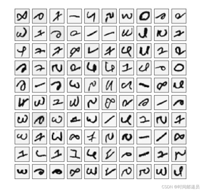

向量化逻辑回归

        我们将使用多个one-vs-all(一对多)logistic回归模型来构建一个多类分类器，由于有10个类，我们需要训练10个独立的分类器。为了提高训练效率，我们采用向量化来解决问题，在本节中，我们将实现一个不使用任何for循环的向量化的logistic回归版本。

向量化代价函数

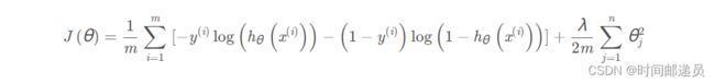
我们将从编写代价函数的一个向量化版本开始，回想一下，在正则化的逻辑回归中，代价函数为：

首先我们对每个样本 要计算下列函数：

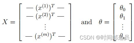
事实上我们可以对所有的样本用矩阵乘法来快速的计算，让我们如下来定义 X 和 θ ：

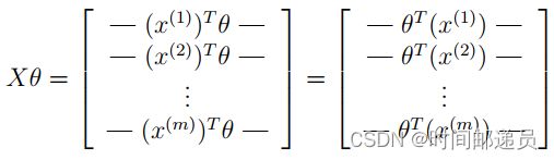
然后通过计算矩阵积 Xθ，我们可以得到：

def sigmoid(z):
    return 1 / (1 + np.exp(-z))

def regularized_cost(theta, X, y, l):
    """
    don't penalize theta_0
    args:
        X: feature matrix, (m, n+1) # 插入了x0=1
        y: target vector, (m, )
        l: lambda constant for regularization
    """
    thetaReg = theta[1:]
    first = (-y*np.log(sigmoid(X@theta))) + (y-1)*np.log(1-sigmoid(X@theta))
    reg = (thetaReg@thetaReg)*l / (2*len(X))
    return np.mean(first) + reg

 向量化梯度

回顾前面的正则化梯度下降：

所以梯度表示如下：

def regularized_gradient(theta, X, y, l):
    """
    don't penalize theta_0
    args:
        l: lambda constant
    return:
        a vector of gradient
    """
    thetaReg = theta[1:]
    first = (1 / len(X)) * X.T @ (sigmoid(X @ theta) - y)
    # 这里人为插入一维0，使得对theta_0不惩罚，方便计算
    reg = np.concatenate([np.array([0]), (l / len(X)) * thetaReg])
    return first + reg

一对多分类器

        这部分我们将实现一对多分类，对于这个任务，我们有10个可能的类，并且由于logistic回归只能一次在2个类之间进行分类，每个分类器在“类别 i”和“不是类别 i”之间决定， 我们将把分类器训练包含在一个函数中，该函数计算10个分类器中的每个分类器的最终权重，并将权重返回，shape为(k, (n+1))数组，其中 n 是参数数量

from scipy.optimize import minimize

def one_vs_all(X, y, l, K):
    """generalized logistic regression
    args:
        X: feature matrix, (m, n+1) # with incercept x0=1
        y: target vector, (m, )
        l: lambda constant for regularization
        K: numbel of labels
    return: trained parameters
    """
    all_theta = np.zeros((K, X.shape[1]))  # (10, 401)
    
    for i in range(1, K+1):
        theta = np.zeros(X.shape[1])
        y_i = np.array([1 if label == i else 0 for label in y])
    
        ret = minimize(fun=regularized_cost, x0=theta, args=(X, y_i, l), method='TNC',
                        jac=regularized_gradient, options={'disp': True})
        all_theta[i-1,:] = ret.x
                         
    return all_theta

上述代码思路：首先我们为X添加了一列常数项 1 以计算截距项； 其次我们将y从类标签转换为每个分类器的二进制值（要么是类i，要么不是类i）；然后我们使用SciPy的优化API来最小化每个分类器的代价函数； 最后将优化程序找到的参数分配给参数数组

def predict_all(X, all_theta):
    # compute the class probability for each class on each training instance   
    h = sigmoid(X @ all_theta.T)  # 注意的这里的all_theta需要转置
    # create array of the index with the maximum probability
    # Returns the indices of the maximum values along an axis.
    h_argmax = np.argmax(h, axis=1)
    # because our array was zero-indexed we need to add one for the true label prediction
    h_argmax = h_argmax + 1
    
    return h_argmax

这里的h共5000行10列，每行代表一个样本，每列是预测对应数字的概率，我们取概率最大对应的index加1就是我们分类器最终预测出来的类别，返回的h_argmax是一个array，包含5000个样本对应的预测值

X = np.insert(X, 0, 1, axis=1)
y = y.flatten()
print(X, y)
All_Theta = one_vs_all(X, y, 1, 10)

y_predict=predict(X, All_Theta)
accuracy=np.mean(y_predict==y)
print("accuracy=%.2f%%"%(accuracy*100))

三、神经网络

        在前一部分中，我们实现了多类逻辑回归来识别手写数字。然而，逻辑回归不能形成更复杂的假设，因为它只是一个线性分类器。在该部分练习中，我们将使用相同的训练集实现神经网络来识别手写数字

模型表示

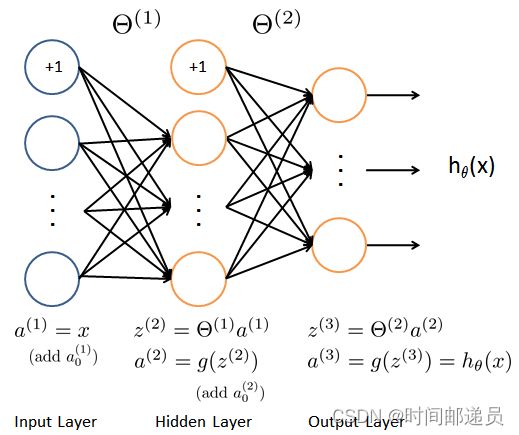
神经网络如图所示，它有3层：输入层、隐藏层和输出层，其中输入是数字图像的像素值

X, y = load_data('ex3data1.mat')
X=np.insert(X,0,1,axis=1)
y=y.flatten()
print(X.shape,y.shape)

前向传播

a1=X
print(a1.shape,Theta1.shape)
[email protected]
print(z2.shape)
z2=np.insert(z2,0,1,axis=1)
a2=sigmoid(z2)
print(a2.shape)
[email protected]
print(z3.shape)
a3=sigmoid(z3)
print(a3)
y_predict=np.argmax(a3,axis=1)+1#返回每行的最大值的索引
print(y_predict.shape)

准确度计算

accuracy=np.mean(y_predict==y)
print("accuracy=%.2f%%"%(accuracy*100))