使用 TensorFlow、Keras-OCR 和 OpenCV 从技术图纸中获取信息
简单介绍
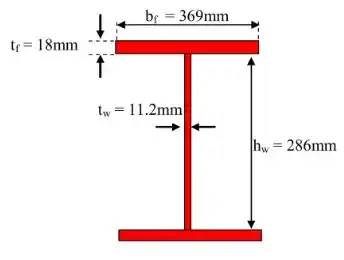
输入是技术绘图图像。对象检测模型获取图像后对其进行分类,找到边界框,分配维度,计算属性。

示例图像(输入)
分类后,找到“IPN”部分。之后,它计算属性,例如惯性矩。它适用于不同类型的部分(IPN、UPN、相等或不相等的支路、组合)。

结果(输出)
你可以从这里查看相关的 github 存储库:https://github.com/ramazanaydinli/Steel-AI/tree/main/final
摘要
这项工作的目的是从与钢结构相关的技术图纸中获取尺寸信息。然而,本文的目的是解释工作的细节,任何感兴趣的人都可以理解背后的想法,并使用类似的技术来解决他们的问题。它仅涵盖一些案例,以证明可以将计算机视觉方法应用于该领域。如果你需要,可以在之后进行一些改进。
要求
深度学习
你必须至少了解一种深度学习框架。就个人而言,使用 TensorFlow,但其他人(例如 PyTorch)也可以完成这项工作。如果你想学习 TensorFlow ,建议:
TensorFlow 简介:https://www.coursera.org/learn/introduction-tensorflow
Tensorflow 高级技术:https://www.coursera.org/specializations/tensorflow-advanced-techniques
光学字符识别
有许多可用的光学字符识别工具,请确保根据你的目标选择最合适的工具。在备选方案中,Keras-OCR 和 Tesseract-OCR 是最受欢迎的。但由于 Tesseract 不支持自定义训练,我们将使用Keras(此功能的优势将在本文的后期详细介绍)。
OpenCV
我相信官方文档绰绰有余,但你需要了解更多信息。
介绍
如果你是一名土木工程师,对你来说,下图应该比较容易看懂。但是考虑到不是每个人都有这方面的知识,在这里提供简单的描述,以便非土木工程师可以看到他们的领域与这个领域之间的相似之处,使用相同的技术,通过稍微调整代码来解决他们的问题。

简单描述一下:你可能会以文本或图像的形式,得到不同的形状、材料或属性,你需要根据这个给定的数据计算指定的属性。
所有的计算都是按规格规范化的,所以如果你知道你需要计算什么,你就可以猜出该计算需要哪些属性。
我们该怎么做?
阅读问题
首先我们需要阅读问题。此时,使用任何OCR读取文本并提取所需内容非常容易。以下示例将帮助你理解:

为简单起见,输入图像被裁剪
上图是我们的输入。我们将使用 Keras-OCR 通过使用下面的代码块来阅读文本:
import keras_ocr

image_path = "Path of the image" # Something like C:\..\image.png
pipeline = keras_ocr.pipeline.Pipeline()
image = keras_ocr.tools.read(image_path)
prediction = pipeline.recognize([image])[0]
boxes = [value[1] for value in prediction]
canvas = keras_ocr.tools.drawBoxes(image=image, boxes=boxes, color=(255, 0, 0), thickness=1)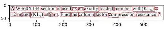
阅读结果
此外,我们可以使用以下方式访问图像的内容:
for text, box in prediction:
    print(text)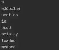
文本的输出
我觉得思路很清晰。你将图像提供给 ocr,ocr 读取它并将输出返回给你。之后我们可以处理这个输出来学习属性。
NLP(自然语言处理——机器阅读文本、理解文本并返回响应)不是这里的主要主题,因此在本文中我们不会对其进行详细介绍,但我们可以使用简单的正则表达式方法将关键字与值匹配。
如果你听说过 ChatGPT——一种最近非常流行的高级聊天机器人,你可以猜到将文本理解为机器并不是这里的大问题。
到目前为止,我们为与读数相关的假设提供了一些基础。接下来我们需要为我们的对象检测做一些准备。
对象检测
我们需要识别绘图和获取尺寸
由于我们在前一部分从文本中获取了信息,因此我们继续分析绘图。但在继续之前,请先看看这篇文章:https://arxiv.org/ftp/arxiv/papers/2205/2205.02659.pdf
我们可以看到,更复杂的绘图在形状和注释方面的识别准确率为 80%。要点是:
Faster-RCNN ResNet50为绘图识别提供了良好的结果。
由于这类作品缺乏数据,人工生成图像是个好主意。
由于支持自定义训练,Keras-OCR非常适合此类工作。例如,如果我们想做一些与基础工程相关的项目,我们需要训练 Keras 学习普通 ocr 目前不知道的地下水位符号。
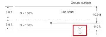
GWT 级别的字符(红色框内)
根据这些信息,下一步是生成人工数据。PIL(Python 图像库)用于此目的。使用此工具,可以创建包含注释的形状。同样,使用最简单的方法,每个形状都是由不同数量的矩形组成的。
创建了三个不同的主要形状。将这些形状彼此相加称为“组合”形状。如果要检查,可以使用此链接访问代码:https://github.com/ramazanaydinli/Steel-AI/blob/main/final/data_generator.py
下面给出了代码生成的一些示例:
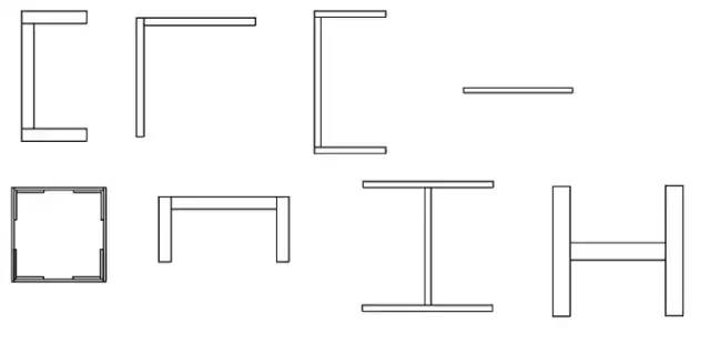
没有注释的形状
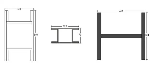
带注释的形状
创建数据后,下一步是安装对象检测环境。按照此处的说明进行操作:https://tensorflow-object-detection-api-tutorial.readthedocs.io/en/latest/install.html
这一步可能出现的错误:
ImportError: cannot import name ‘builder’ from ‘google.protobuf.internal’
由于某种原因,此文件已从官方安装文件中删除。从这里(https://raw.githubusercontent.com/protocolbuffers/protobuf/main/python/google/protobuf/internal/builder.py)复制原始文件。创建 builder.py 文件,将原始代码粘贴到其中,保存文件,然后将文件移动到:{your_environment_location}/site-packages/google/protobuf/internal/builder.py
下一步是使用 ResNet50 的推理进行自定义对象检测训练。按照此处的说明进行操作:https://tensorflow-object-detection-api-tutorial.readthedocs.io/en/latest/training.html
直到到达“下载预训练模型”部分。在这部分中,我们将下载 FasterRCNN-ResNet50 640x640 而不是 SSD_ResNet50。应严格遵守其余说明。
这一步可能出现的错误:
UTF-8 codec can’t decode …
如果你得到 UTF-8 错误,你应该注意 pbtxt 文件的扩展名,再次检查它。
为简单起见,我们将使用三种不同的形状:
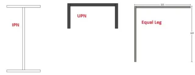
上面的形状将输入模型
item {
    id: 1
    name: 'IPN'
}

item {
    id: 2
    name: 'Legged'
}

item {
    id: 3
    name: 'UPN'
}
所以我们的 label_map.pbtxt 文件应该和上面一样。
同样在 pipeline.config 文件中,更改:
...
num_classes = 3 #default value is 90
...

train_config: {
  batch_size: 64  # Lower this value if your computer gave memory error
  sync_replicas: true
  startup_delay_steps: 0
  replicas_to_aggregate: 8
  num_steps: 25000 # It is up to you but this kind of simple drawings even 2000 could get the job done
  optimizer {
    momentum_optimizer: {
      learning_rate: {
        cosine_decay_learning_rate {
          learning_rate_base: .04
          total_steps: 25000   # If you changed previous value, change this value too
          warmup_learning_rate: .013333
          warmup_steps: 2000 # Arrange warmup steps, change it into %10 of num_steps
        }
      }
      momentum_optimizer_value: 0.9
    }
    use_moving_average: false
  }
  fine_tune_checkpoint_version: V2
  fine_tune_checkpoint: "PATH_TO_BE_CONFIGURED" #Specify the path of ckpt-0 file
  fine_tune_checkpoint_type: "classification" # Change this value into "detection"
  data_augmentation_options {
    random_horizontal_flip {
    }
  }

...
train_input_reader: {
  label_map_path: "PATH_TO_BE_CONFIGURED/label_map.txt" # Specify the path of label_map
  tf_record_input_reader {
    input_path: "PATH_TO_BE_CONFIGURED/train2017-?????-of-00256.tfrecord" #Specify the path of training tf.record files you created with protobuff
  }
}
...

eval_input_reader: {
  label_map_path: "PATH_TO_BE_CONFIGURED/label_map.txt" #Again specify label map path
  shuffle: false
  num_epochs: 1
  tf_record_input_reader {
    input_path: "PATH_TO_BE_CONFIGURED/val2017-?????-of-00032.tfrecord" #Specify the path of testing tf.record files you created with protobuff
  }
}
如果你在这一步之前所做的一切都正确,你就可以开始训练,这需要一些时间。更强的 GPU 需要更短的训练时间,你也可以调整 pipeline.config 文件中的“step_size”参数来缩短它。更改参数时注意不要过拟合或欠拟合。
图像处理
假设一切正常,我们就可以开始处理图像了。Jupter Notebook 将用于后续步骤。我们将从导入所需的库开始。
import os
os.environ['TF_CPP_MIN_LOG_LEVEL'] = '2'    # Suppress TensorFlow logging (1)
import pathlib
import tensorflow as tf

tf.get_logger().setLevel('ERROR')           # Suppress TensorFlow logging (2)

# Enable GPU dynamic memory allocation
gpus = tf.config.experimental.list_physical_devices('GPU')
for gpu in gpus:
    tf.config.experimental.set_memory_growth(gpu, True)
main_path=os.getcwd()
新建一个目录,粘贴一张图片进去测试,如果需要可以多拍几张。采取它在 jupter 中使用该图像的路径。
image_paths = []
for image_name in os.listdir("{your directory path}"):
    image_paths.append(os.path.join("{your directory path}", image_name))
上面的循环将获取该目录中的每个图像并获取图像路径。
MODEL_DATE = '20221206'
MODEL_NAME = 'my_resnet'
LABEL_FILENAME = 'label_map.pbtxt'
PATH_TO_LABELS = os.path.join(main_path, "annotations", LABEL_FILENAME)
PATH_TO_MODEL_DIR = os.path.join(main_path, "models")
PATH_TO_CFG = os.path.join(PATH_TO_MODEL_DIR, "my_resnet", "pipeline.config" )
PATH_TO_CKPT = os.path.join(PATH_TO_MODEL_DIR, "my_resnet")
上面的代码块是兼容性所必需的。
import time
from object_detection.utils import label_map_util
from object_detection.utils import config_util
from object_detection.utils import visualization_utils as viz_utils
from object_detection.builders import model_builder


print('Loading model... ', end='')
start_time = time.time()

# Load pipeline config and build a detection model
configs = config_util.get_configs_from_pipeline_file(PATH_TO_CFG)
model_config = configs['model']
detection_model = model_builder.build(model_config=model_config, is_training=False)

# Restore checkpoint
ckpt = tf.compat.v2.train.Checkpoint(model=detection_model)
ckpt.restore(os.path.join(PATH_TO_CKPT, 'ckpt-3')).expect_partial()

@tf.function
def detect_fn(image):
    """Detect objects in image."""

    image, shapes = detection_model.preprocess(image)
    prediction_dict = detection_model.predict(image, shapes)
    detections = detection_model.postprocess(prediction_dict, shapes)

    return detections

end_time = time.time()
elapsed_time = end_time - start_time
print('Done! Took {} seconds'.format(elapsed_time))
上面,我们导入了所需的模块并加载了我们之前训练的模型。
category_index = label_map_util.create_category_index_from_labelmap(PATH_TO_LABELS,
use_display_name=True)
def load_image_into_numpy_array(path):
"""Load an image from file into a numpy array.
Puts image into numpy array to feed into tensorflow graph.
Note that by convention we put it into a numpy array with shape
(height, width, channels), where channels=3 for RGB.
Args:
path: the file path to the image
Returns:
uint8 numpy array with shape (img_height, img_width, 3)
"""
return np.array(Image.open(path))
for image_path in image_paths:
print('Running inference for {}... '.format(image_path), end='')
image_np = load_image_into_numpy_array(image_path)
img_height, img_width = image_np.shape[0], image_np.shape[1]
input_tensor = tf.convert_to_tensor(np.expand_dims(image_np, 0), dtype=tf.float32)
detections = detect_fn(input_tensor)
# All outputs are batches tensors.
# Convert to numpy arrays, and take index [0] to remove the batch dimension.
# We're only interested in the first num_detections.
num_detections = int(detections.pop('num_detections'))
detections = {key: value[0, :num_detections].numpy()
for key, value in detections.items()}
detections['num_detections'] = num_detections
# detection_classes should be ints.
detections['detection_classes'] = detections['detection_classes'].astype(np.int64)
label_id_offset = 1
image_np_with_detections = image_np.copy()
viz_utils.visualize_boxes_and_labels_on_image_array(
image_np_with_detections,
detections['detection_boxes'],
detections['detection_classes']+label_id_offset,
detections['detection_scores'],
category_index,
use_normalized_coordinates=True,
max_boxes_to_draw=200,
min_score_thresh=0.3,
agnostic_mode=False)
plt.figure()
plt.imshow(image_np_with_detections)
print('Done')
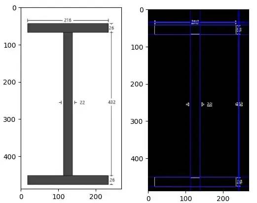
plt.show()此时你应该看到对象检测结果,即标签和边界框坐标。这里有几个示例结果:

使用边界框检测 IPN 形状

网上随便找的一张图(连手绘都认得)

Equal Leg标签和bounding box检测结果

左图是1个IPN和1个UPN的组合图,中间和右边的图是网上的随机图,以前没见过这个模型,但是label和bounding boxes还是可以用的
通过这些测试图像,我们可以说我们的模型可以很好地预测标签和指定边界框。
下一步是从这些图像中获取尺寸。我们会将边界框内部与图像的其余部分隔离开来,这样我们就可以轻松地对其进行处理。
boxes = detections['detection_boxes']

# get all boxes from an array
max_boxes_to_draw = boxes.shape[0]

# get scores to get a threshold
scores = detections['detection_scores']

# this is set as a default but feel free to adjust it to your needs
min_score_thresh=.5

# iterate over all objects found
for i in range(min(max_boxes_to_draw, boxes.shape[0])):
    if scores is None or scores[i] > min_score_thresh:
        # boxes[i] is the box which will be drawn
        class_name = category_index[detections['detection_classes'][i+1]]['name']
        print ("This box is gonna get used", boxes[i], detections['detection_classes'][i+1])
可以从上面的代码块中找到边界框坐标。需要注意的重要一点是,模型检测到许多边界框,但我们将使用最大的一个。我们还向“i”添加了“1”,因为我们的标签映射从 1 开始,而循环从 0 开始。
top_y = boxes[0][0]*img_height
left_x = boxes[0][1]*img_width
bottom_y = boxes[0][2]*img_height
right_x = boxes[0][3]*img_width
我们分离了边界框的像素值。
由于我们知道标签(IPN、UPN 或 Leg)和边界框坐标,我们可以处理图像以获得尺寸。这里可以使用几种不同的方法。
import cv2
import math
image_path = image_paths[0]
img = cv2.imread(image_path)
extra_pixels = 5
y_top = int(top_y)-extra_pixels
y_bottom = int(bottom_y)+extra_pixels
x_left = int(left_x) - extra_pixels
x_right = int(right_x) + extra_pixels
roi = img[y_top:y_bottom,x_left:x_right]

#Hough Line
dst = cv2.Canny(roi, 50, 200, None, 3)
cdst = cv2.cvtColor(dst, cv2.COLOR_GRAY2BGR)
lines = cv2.HoughLines(dst, 1, np.pi/180, 150, None, 0,0)
line_points = []

if lines is not None:
       for i in range(0, len(lines)):
            rho = lines[i][0][0]
            theta = lines[i][0][1]
            a = math.cos(theta)
            b = math.sin(theta)
            x0 = a * rho
            y0 = b * rho
            pt1 = (int(x0 + 1000*(-b)), int(y0 + 1000*(a)))
            pt2 = (int(x0 - 1000*(-b)), int(y0 - 1000*(a)))
            line_points.append([pt1, pt2])
            cv2.line(cdst, pt1, pt2, (0,0,255), 1, cv2.LINE_AA)
plt.imshow(cdst)


# Probabilistic Hough Line
# edges = cv2.Canny(roi, 50, 150, apertureSize=3)
# linesP = cv2.HoughLinesP(edges, 1, np.pi/180, 50, 100, 2)
# if linesP is not None:
#    for i in range(0, len(linesP)):
#        l = linesP[i][0]
#        cv2.line(roi, (l[0], l[1]), (l[2], l[3]), (0,0,255), 1, cv2.LINE_AA)
# cv2.imwrite("roi.png", roi)
# plt.imshow(roi)
限制
用于这种情况的明显方法是霍夫线。但问题是,正常的霍夫变换和概率霍夫变换都无法检测短线,也就是注释的边界。查看以下示例:
左 — roi,裁剪图像(感兴趣区域),右 — roi 的霍夫线结果
如你所见,检测到所有长线,但未检测到短线。Probabilistic HLine 结果也有同样的问题,查看下图:
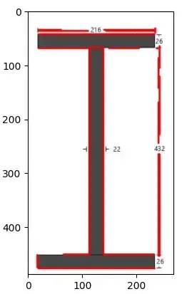
如果我们可以获得与长线一起的短线,我们可以将霍夫线坐标与注释边界坐标相匹配。使用一些规则(if-else 块),可以获得非常好的结果。
另一个问题是,通常形状都带有注释,但有时整个形状可以用特定的名称来描述(例如只给出名称“HE300A”,属性应该从部分表中获取),但是几个 if-else 块可以工作。
考虑到整体的局限性和可能性,目前最好的方法是通过区域坐标进行匹配。
import keras_ocr
roi_path = os.path.join(main_path, "roi.png")
pipeline = keras_ocr.pipeline.Pipeline()

image = keras_ocr.tools.read(roi_path)
prediction = pipeline.recognize([image])[0]
boxes = [value[1] for value in prediction]

canvas = keras_ocr.tools.drawBoxes(image=image, boxes=boxes, color=(255, 0, 0), thickness=1)
Keras 读取结果
对于上面的示例,我们获得了所有尺寸及其边界框。计算出边界框后,我们可以将它们放入一个区域并根据该区域进行匹配。
annot_centers = []
readings = [value[0] for value in prediction]
value_center_list = []

for box in boxes:
    x_center = []
    y_center = []
    x_sum = 0
    y_sum = 0
    for point in box:
        x_sum += point[0]
        y_sum += point[1]
    x_center = int(x_sum/4)
    y_center = int(y_sum/4)
    value_center_list.append([x_center, y_center])

for i in range(len(value_center_list)):
    value_center_list[i].append(readings[i])
简而言之,我们假设 y 轴注释位于左四分之一或右四分之一。x 轴注释的方法相同,如果它位于顶部或底部四分之一,我们可以假设它与 x 轴相关。
唯一的例外是中间,如果它的位置不在上述任何区域中,我们将指定该读数作为腹板厚度。
最后,下面的代码块根据分配的属性进行计算。
# Moment of inertia calculations
total_shape_area = (t_web*h_web) + (top_t_flange * b_flange) + (bottom_t_flange * b_flange)

# Datum assumed as top left of the shape
# Strong axis will be taken as x axis, so week axis will be y axis
area_moments_x = (top_t_flange * b_flange) * (top_t_flange/2) + (t_web*h_web)*(h_web/2 + top_t_flange)+ (bottom_t_flange * b_flange) * (top_t_flange + h_web + bottom_t_flange/2)
center_of_gravity_x = area_moments_x / total_shape_area
area_moments_y = (top_t_flange * b_flange) * (b_flange/2) + (t_web*h_web)*(b_flange/2)+ (bottom_t_flange * b_flange) * (b_flange/2)
center_of_gravity_y = area_moments_y / total_shape_area

# These values are obvious for symmetrical shapes, but just for different cases these should be calculated
moment_of_inertia_x = (1/12) * b_flange * top_t_flange**3 + (top_t_flange * b_flange) * (center_of_gravity_x - top_t_flange/2)**2 + (1/12)* t_web * h_web**3 + (t_web * h_web) * (center_of_gravity_x - (top_t_flange + h_web/2))**2 + (1/12) * b_flange * bottom_t_flange**3 + (b_flange * bottom_t_flange) * ((top_t_flange + h_web + bottom_t_flange/2) - center_of_gravity_x)**2
结果
我们可以使用深度学习和图像处理技术解决钢结构问题,但需要一定的投资。还有其他类型的图纸可以处理,但由于时间和精力所限,这里就不一一列举了。通过一些更改,这项工作可以应用于许多不同的领域。
参考
https://arxiv.org/ftp/arxiv/papers/2205/2205.02659.pdf
https://arxiv.org/pdf/1506.01497.pdf
☆ END ☆
如果看到这里,说明你喜欢这篇文章,请转发、点赞。微信搜索「uncle_pn」,欢迎添加小编微信「 woshicver」,每日朋友圈更新一篇高质量博文。
↓扫描二维码添加小编↓
