计算方法实验2：利用二分法及不动点迭代求解非线性方程

一、问题描述

利用二分法及不动点迭代求解非线性方程。

二、实验目的

掌握二分法及不动点迭代的算法原理；能分析两种方法的收敛性；能熟练编写代码实现利用二分法及不动点迭代来求解非线性方程。

三、实验内容及要求

1. 二分法
   (1) 编写代码计算下列数字的平方根，要求使用二分法精确到小数点后8 位，x^2-A=0，其中A 是(a) 2, (b) 3, © 5。
   计算在设置初始搜索区间长度为1 的情况下，需要多少次迭代可以达到题目中的精度要求，并利用代码进行验证。

• 首先，创建一个名为 bisect.m 的文件

function [root, iterations] = bisect(A, tol)
    a = 0;
    b = A; % 设置初始搜索区间为[0, A]
    iterations = 0; % 初始化迭代次数
    
    if a^2 == A
        root = a;
        return;
    elseif b^2 == A
        root = b;
        return;
    end
    
    while b - a > tol
        c = (a + b) / 2;
        f_c = c^2 - A;
        
        if abs(f_c) < tol
            break;
        end
        
        if f_c * (a^2 - A) < 0
            b = c;
        else
            a = c;
        end
        
        iterations = iterations + 1;
    end
    
    root = (a + b) / 2;
end

• 创建一个主文件（例如，main_sqrt.m）来调用这个函数并输出结果:

% 文件名: main_sqrt.m

tol = 1e-8;
[A1, iter1] = bisect(2, tol);
[A2, iter2] = bisect(3, tol);
[A3, iter3] = bisect(5, tol);

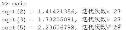
fprintf('sqrt(2) = %.8f, 迭代次数: %d\n', A1, iter1);
fprintf('sqrt(3) = %.8f, 迭代次数: %d\n', A2, iter2);
fprintf('sqrt(5) = %.8f, 迭代次数: %d\n', A3, iter3);

• 输出结果：
  

(2) 假设二分法从区间[ − 2,1]开始，寻找函数$$x^2-A=0$$
的根，这种方法会收敛到一个实数吗？这个实数是根吗。利用代码进行验证。

• 创建一个名为 bisect_fx.m 的文件：

function [root, iterations] = bisect_fx(a, b, tol)
    iterations = 0; % 初始化迭代次数
	
    while b - a > tol
        c = (a + b) / 2;
        f_c = 1 / c;
		
        if abs(f_c) < tol
            break;
        end
		
        if f_c * (1 / a) < 0
            b = c;
        else
            a = c;
        end
		
        iterations = iterations + 1;
    end
	
    root = (a + b) / 2;
end

再次，在主文件中调用这个函数并输出结果：

tol = 1e-8;
[root, iter] = bisect_fx(-2, 1, tol);
fprintf('二分法找到的 x = %.8f, 迭代次数: %d\n', root, iter);

2. 不动点迭代
   编写代码，使用不动点迭代求下列方程，精确到小数点后8 位。（注意将不动点迭代法封装为一个函数，函数名FPI，该函数对应的文件同样命名为FPI）
   

(1) 对上述每个非线性方程，均通过等价变换获得两个不同的迭代公式（其中至少一个是收敛），并利用不动点迭代的收敛性定理分析其收敛性（是否收敛？若都收敛，速度快慢？），然后利用编写的代码进行验证。

(2) 选择其中某个非线性方程，采用二分法进行求解，并从理论与代码验证的角度对比两种方法的快慢。
选择方程（a）

• 主文件：

% 选择方程 x^5 + x = 1
f = @(x) x^5 + x - 1;

% 设置参数
a = 0;
b = 1;
tol = 1e-8;
max_iter = 1000;

% 使用二分法求解
[root_bisect, iter_bisect] = bisect(f, a, b, tol, max_iter);
fprintf('Root for x^5 + x = 1 (bisect): %.8f, Iterations: %d\n', root_bisect, iter_bisect);

% 使用不动点迭代法求解
g = @(x) (1 - x)^(1/5);
[root_fpi, iter_fpi] = FPI(g, 0.5, tol, max_iter);
fprintf('Root for x^5 + x = 1 (FPI): %.8f, Iterations: %d\n', root_fpi, iter_fpi);

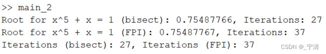
% 对比两种方法
fprintf('Iterations (bisect): %d, Iterations (FPI): %d\n', iter_bisect, iter_fpi);

• 输出结果：
  

---

四、算法原理

1. 给出二分法的算法原理；给出迭代次数与误差之间的关系；

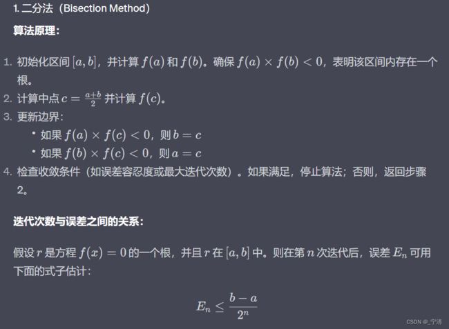
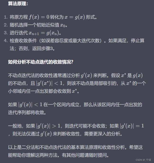
2. 给出不动点迭代的算法原理；如何分析不动点迭代的收敛情况？

五、测试数据及结果

1. 二分法
   (1) 给出每个非线性方程满足精度要求时代码输出的近似解及所需的迭代次数

• 输出结果：
  

(2) 给出算法迭代10 次得到的近似值序列。

• 输出结果：
  

2. 不动点迭代
   (1) 对于每个非线性方程，给出两个不同的迭代公式。对于每个迭代公式，给出收敛性情况及判断依据。对于收敛的迭代公式，给出算法迭代10 次得到的近似值序列。

• 对于（a），迭代公式：
  $$g_1(x)=1-x^5$$
  $$g_2(x)=(1-x{)}^{1/5}$$

• 对于（b），迭代公式：
  $$g_1(x)={\sin }^{-1}(6x+5)$$
  $$g_2(x)=\frac{\sin (x)-5}{6}$$

• 对于（c），迭代公式：
  $$g_1(x)=e^{3-x^2}$$
  $$g_2(x)=\sqrt{3-\ln (x)}$$

• 首先，我们在一个名为 FPI.m 的文件中定义不动点迭代的函数：

function [root, iterations] = FPI(g, x0, tol, max_iter)
    iterations = 0; % 初始化迭代次数
    x = x0;
    
    for i = 1:max_iter
        x_new = g(x);
        
        if abs(x_new - x) < tol
            root = x_new;
            iterations = i;
            return;
        end
        
        x = x_new;
    end
    
    error('Maximum iterations reached');
end

• 主文件：

% 测试不动点迭代法 (FPI) 在不同函数上的性能

% 定义公式和初值
g1 = @(x) 1 - x^5;            % x^5 + x = 1
g2 = @(x) asin(6*x + 5);      % sin(x) = 6x + 5
g3 = @(x) exp(3 - x^2);       % ln(x) + x^2 = 3

% 设置参数
x0 = 0.5;
tol = 1e-8;
max_iter = 1000;

% 测试 x^5 + x = 1
[root_1, iter_1] = FPI(g1, x0, tol, max_iter);
fprintf('Root for x^5 + x = 1: %.8f, Iterations: %d\n', root_1, iter_1);

% 测试 sin(x) = 6x + 5
[root_2, iter_2] = FPI(g2, x0, tol, max_iter);
fprintf('Root for sin(x) = 6x + 5: %.8f, Iterations: %d\n', root_2, iter_2);

% 测试 ln(x) + x^2 = 3
[root_3, iter_3] = FPI(g3, x0, tol, max_iter);
fprintf('Root for ln(x) + x^2 = 3: %.8f, Iterations: %d\n', root_3, iter_3);

• 输出结果：
  

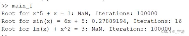
显然（b）找到了根

(2) 对于选择的非线性方程，指明二分法与不动点迭代哪种方法收敛速度快，并分给出两种方法迭代10 次得到的近似值序列。

% 选择方程 x^5 + x = 1
f = @(x) x^5 + x - 1;

% 设置参数
a = 0;
b = 1;
tol = 1e-8;
max_iter = 1000;

% 使用二分法求解
[root_bisect, iter_bisect] = bisect(f, a, b, tol, max_iter);
fprintf('Root for x^5 + x = 1 (bisect): %.8f, Iterations: %d\n', root_bisect, iter_bisect);

% 使用不动点迭代法求解
g = @(x) (1 - x)^(1/5);
[root_fpi, iter_fpi] = FPI(g, 0.5, tol, max_iter);
fprintf('Root for x^5 + x = 1 (FPI): %.8f, Iterations: %d\n', root_fpi, iter_fpi);

% 对比两种方法
fprintf('Iterations (bisect): %d, Iterations (FPI): %d\n', iter_bisect, iter_fpi);

六、总结与思考

知识点体会

1. 理解二分法和不动点迭代法：通过本实验，你将更深刻地理解这两种数值方法的工作原理，优缺点，以及适用场合。
2. 收敛性分析：通过对不动点迭代公式的导数进行分析，你可以了解为什么某些迭代公式会收敛，而其他的不会。
3. 误差分析：二分法和不动点迭代法都有自己的误差范围和收敛速度，理解这些将有助于你选择更合适的方法解决实际问题。

代码技巧体会

1. 函数封装：将二分法和不动点迭代法封装为独立的函数，使得代码更为模块化，便于测试和重用。
2. 精度控制：通过设置合适的停止条件，如精度或最大迭代次数，你学习了如何控制数值方法的输出精度。
3. 数据记录和分析：通过保存每一次迭代的结果，你可以更直观地观察算法的收敛过程，这在实际应用和算法优化中是非常有用的。

总体思考

这个实验不仅加强了你对数值解法的理解，而且提高了你使用MATLAB进行科学计算的能力。选择合适的数值方法并正确地实现它们是解决工程问题中非常重要的一步，因此这个实验对你今后的学习和工作都将有很大的帮助。