(一)单细胞数据分析——单细胞数据预处理
由于毕业设计是单细胞数据的处理,所以把整个过程所用到的方法进行一个整理,这是第一个部分,对得到的单细胞数据进行质控、降维、聚类等预处理。下面开始:
第一步:导入R包(部分R包可能用不到,因为做课题的时候需要就全部导入了,无伤大雅!)
library(scibet)
library(Seurat)
library(scater)
library(scran)
library(dplyr)
library(Matrix)
library(cowplot)
library(ggplot2)
library(harmony)
rm(list = ls())
第二步:读入所需要的数据
这里是我使用的一个乳腺癌单细胞测序数据
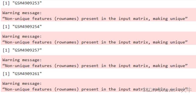
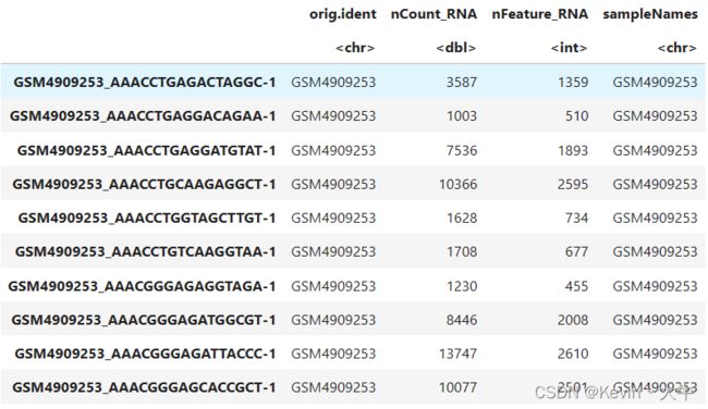
file.dir <- './GSE161529_RAW'
samplefile <- list.files('./GSE161529_RAW')
samplefile.mtx <- samplefile[grepl(pattern = 'matrix.mtx.gz',x = samplefile)]
samplefile.barcodes <- samplefile[grepl(pattern = 'barcodes.tsv.gz',x = samplefile)]
names(samplefile.mtx) <- substr(x = samplefile.mtx,start = 1,stop = 10)
names(samplefile.barcodes) <- substr(x = samplefile.barcodes,start = 1,stop = 10)
feature.file <- 'GSE161529_features.tsv.gz'
feature.names <- read.table(file = feature.file, header = FALSE, sep = "\t", row.names = NULL)
select_data <- c("GSM******") #这里的******指的是样本编号
GSE161529List <- lapply(select_data, function(sampleName){
    print(sampleName)
    tmp.barcode <- paste(file.dir, samplefile.barcodes[sampleName], sep = "/")
    tmp.mtx <- paste(file.dir, samplefile.mtx[sampleName], sep = "/")
    cell.barcodes <- read.table(file = tmp.barcode, header = FALSE, sep = "\t", row.names = NULL)
    data <- readMM(file = tmp.mtx)
    colnames(data) <- cell.barcodes[,1]
    rownames(data) <- feature.names[,2]
    CreateSeuratObject(counts = data, project = sampleName)
})
names(GSE161529List) <- select_data
BRCA_GSE161529 <- merge(GSE161529List[[1]], GSE161529List[-1], add.cell.ids = names(GSE161529List))
BRCA_GSE161529$sampleNames <- BRCA_GSE161529$orig.ident
head(BRCA_GSE161529)
当出现以下弹出消息则表示正在读入:
最终head()的结果如下:
第三步:质量控制、细胞周期异质性减弱与细胞的降维聚类
因为这些步骤都是普遍通用的,这里封装为SeuratPreTreatment()方法,通过四个质控指标nCount_RNA(每个细胞的read counts数目)≥500、nFeature_RNA(每个细胞所检测到的基因数目) ≥200、mitoRatio(线粒体基因比例)<0.2、GenesPerUMI(单位read counts检测到的基因数目的比例)>0.8,进行质量控制;使用CellCycleScoring()减弱细胞周期异质性对下游分析的影响;之后就是标化、降维PCA/Harmony(Harmony是针对需要消除批次效应时使用,不一定都要使用)与聚类。
SeuratPreTreatment <- function(obj=NULL,QC=FALSE,nCount_cut=500,nFeature_cut=200,log10GenesPerUMI_cut=0.8,mitoRatio_cut=0.2){
    if(is.null(obj)){
        print("obj is null!")
        return(NULL)
    }
    obj$mitoRatio <- PercentageFeatureSet(object = obj, pattern = "^MT-")
    obj$mitoRatio <- [email protected]$mitoRatio / 100
    obj$log10GenesPerUMI <- log10(obj$nFeature_RNA)/log10(obj$nCount_RNA)
    obj$riboRatio <- PercentageFeatureSet(object = obj, pattern = "^RP[SL]")
    obj$riboRatio <- [email protected]$mitoRatio / 100
    obj <- CellCycleScoring(obj, g2m.features = g2m_genes, s.features = s_genes)
    if(QC){
        filtered_obj <- subset(x = obj, subset= (nCount_RNA >= nCount_cut) &
                               (nFeature_RNA >= nFeature_cut) &
                               (log10GenesPerUMI > log10GenesPerUMI_cut) &
                               (mitoRatio < mitoRatio_cut))
        print(dim(filtered_obj))
        filtered_obj <- NormalizeData(filtered_obj, normalization.method = "LogNormalize")
        filtered_obj <- FindVariableFeatures(filtered_obj, selection.method = "vst", nfeatures = 3000)
        filtered_obj <- ScaleData(filtered_obj, vars.to.regress = c('nCount_RNA'))
        filtered_obj <- RunPCA(filtered_obj)
        filtered_obj <- RunUMAP(filtered_obj,reduction = "pca",dims = 1:30,seed.use = 12345)
        filtered_obj <- FindNeighbors(filtered_obj,reduction = 'pca', dims = 1:30, verbose = FALSE)
        filtered_obj <- FindClusters(filtered_obj,resolution = 0.5, verbose = FALSE,random.seed=20220727)
        return(filtered_obj)
    }else{
        obj <- NormalizeData(obj, normalization.method = "LogNormalize")
        obj <- FindVariableFeatures(obj, selection.method = "vst", nfeatures = 3000)
        obj <- ScaleData(obj, vars.to.regress = c('nCount_RNA'))
        obj <- RunPCA(obj)
        obj <- RunUMAP(obj,reduction = "pca",dims = 1:30,seed.use = 12345)
        obj <- FindNeighbors(obj,reduction = 'pca', dims = 1:30, verbose = FALSE)
        obj <- FindClusters(obj,resolution = 0.5, verbose = FALSE,random.seed=20220727)
        return(obj)
    }
}
方法封装完成后,质控参数QC设置为TRUE,使用该方法预处理数据
BRCA_GSE161529_QC <- SeuratPreTreatment(BRCA_GSE161529, QC = TRUE)
第四步:细胞注释
使用经典的细胞代表的基因集对数据进行注释,基因集详见代码;同时将细胞注释的代码封装为方法cellAnnotation()
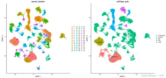
cellAnnotation <- function(obj,markerList,assay='SCT',slot='data'){
    markergene <- unique(do.call(c,markerList))
    Idents(obj) <- 'seurat_clusters'
    cluster.averages <- AverageExpression(obj,assays=assay, slot = slot,features=markergene, return.seurat = TRUE)
    if(assay=='SCT'){
        scale.data <- cluster.averages@assays$SCT@data
    }else{
        scale.data <- cluster.averages@assays$RNA@data
    }
    print(scale.data)
    cell_score <- sapply(names(markergeneList),function(x){
        tmp <- scale.data[rownames(scale.data)%in%markergeneList[[x]],]
        if(is.matrix(tmp)){
            if(nrow(tmp)>=2){
                res <- apply(tmp,2,max)
                return(res)
            }else{
                return(rep(-2,ncol(tmp)))
            }
        }else{
            return(tmp)
        }
    })
    print(cell_score)
    celltypeMap <- apply(cell_score,1,function(x){
        colnames(cell_score)[which(x==max(x))]
    },simplify = T)
    [email protected]$cellType_auto <- plyr::mapvalues(x = [email protected], from = names(celltypeMap), to = celltypeMap)
    return(obj)
}
lymphocyte <- c('CD3D','CD3E','CD79A','MS4A1','MZB1')
myeloid <- c('CD68','CD14','TPSAB1' , 'TPSB2','CD1E','CD1C','LAMP3', 'IDO1')
EOC <- c('EPCAM','KRT19','CD24')
fibo_gene <- c('DCN','FAP','COL1A2')
endo_gene <- c('PECAM1','VWF')
markergeneList <- list(lymphocyte=lymphocyte,myeloid=myeloid,Epi=EOC,fibo=fibo_gene,endo=endo_gene)
BRCA_GSE161529_QC <- cellAnnotation(obj=BRCA_GSE161529_QC,assay = 'RNA',markerList=markergeneList)
可以通过DimPlot()查看预处理后的单细胞UMAP图
DimPlot(object = BRCA_GSE161529_QC,reduction = 'umap',group.by = c('seurat_clusters','cellType_auto'), label = TRUE)
第五步:存入预处理后的单细胞数据
saveRDS(object = BRCA_GSE161529_QC,file = './BRCA_GSE161529_obj.RDS')
第(一)部分单细胞数据预处理就完成了,之后还有对细胞亚群的分群,伪时序分析等教程哦!关注不迷路!