Selection Sort
The selection sort algorithm sorts an array by repeatedly finding the minimum element (considering ascending order) from unsorted part and putting it at the beginning. The algorithm maintains two subarrays in a given array.
1) The subarray which is already sorted.
2) Remaining subarray which is unsorted.
In every iteration of selection sort, the minimum element (considering ascending order) from the unsorted subarray is picked and moved to the sorted subarray.
void selectionSort(int arr[], int n)
{
    int i, j, min_idx;

    // One by one move boundary of unsorted subarray
    for (i = 0; i < n-1; i++)
    {
        // Find the minimum element in unsorted array
        min_idx = i;
        for (j = i+1; j < n; j++)
          if (arr[j] < arr[min_idx])
            min_idx = j;

        // Swap the found minimum element with the first element
        swap(&arr[min_idx], &arr[i]);
    }
}
Time Complexity: O(n*n) as there are two nested loops.
Auxiliary Space: O(1)
The good thing about selection sort is it never makes more than O(n) swaps and can be useful when memory write is a costly operation.
Insertion Sort
void insertionSort(int arr[], int n)
{
   int i, key, j;
   for (i = 1; i < n; i++)
   {
       key = arr[i];
       j = i-1;

       /* Move elements of arr[0..i-1], that are
          greater than key, to one position ahead
          of their current position */
       while (j >= 0 && arr[j] > key)
       {
           arr[j+1] = arr[j];
           j = j-1;
       }
       arr[j+1] = key;
   }
}
Time Complexity: O(n*n)
Auxiliary Space: O(1)
Boundary Cases: Insertion sort takes maximum time to sort if elements are sorted in reverse order. And it takes minimum time (Order of n) when elements are already sorted.
Algorithmic Paradigm: Incremental Approach
Sorting In Place: Yes
Stable: Yes
Online: Yes
Uses: Insertion sort is uses when number of elements is small. It can also be useful when input array is almost sorted, only few elements are misplaced in complete big array.
Bubble Sort
// An optimized version of Bubble Sort
void bubbleSort(int arr[], int n)
{
   int i, j;
   bool swapped;
   for (i = 0; i < n-1; i++)
   {
     swapped = false;
     for (j = 0; j < n-i-1; j++)
     {
        if (arr[j] > arr[j+1])
        {
           swap(&arr[j], &arr[j+1]);
           swapped = true;
        }
     }

     // IF no two elements were swapped by inner loop, then break
     if (swapped == false)
        break;
   }
}
Worst and Average Case Time Complexity: O(n*n). Worst case occurs when array is reverse sorted.
Best Case Time Complexity: O(n). Best case occurs when array is already sorted.
Auxiliary Space: O(1)
Boundary Cases: Bubble sort takes minimum time (Order of n) when elements are already sorted.
Sorting In Place: Yes
Stable: Yes
Merge Sort
MergeSort(arr[], l,  r)
If r > l
     1. Find the middle point to divide the array into two halves:
             middle m = (l+r)/2
     2. Call mergeSort for first half:
             Call mergeSort(arr, l, m)
     3. Call mergeSort for second half:
             Call mergeSort(arr, m+1, r)
     4. Merge the two halves sorted in step 2 and 3:
             Call merge(arr, l, m, r)
The following diagram shows the complete merge sort process for an example array {38, 27, 43, 3, 9, 82, 10}. If we take a closer look at the diagram, we can see that the array is recursively divided in two halves till the size becomes 1. Once the size becomes 1, the merge processes comes into action and starts merging arrays back till the complete array is merged.
Time Complexity: Sorting arrays on different machines. Merge Sort is a recursive algorithm and time complexity can be expressed as following recurrence relation.
T(n) = 2T(n/2) +
The above recurrence can be solved either using Recurrence Tree method or Master method. It falls in case II of Master Method and solution of the recurrence is .
Time complexity of Merge Sort is in all 3 cases (worst, average and best) as merge sort always divides the array in two halves and take linear time to merge two halves.
Auxiliary Space: O(n)
Algorithmic Paradigm: Divide and Conquer
Sorting In Place: No in a typical implementation
Stable: Yes
Heap Sort
Heapify:
HEAPIFY(A,i)
 1 left <- left(i)
 2 right <- right(i)
 3 if node i has a larger child
 4    then swap A[i] and largest child
 5         HEAPIFY(A,location largest child was in)
BuildHeap:
BUILDHEAP(A)
 1 heapsize <- length(A)
 2 for i <- floor(length(A)/2) downto 1  **lowest parent up to root**
 3     do HEAPIFY(A,i)
HeadSort:
HEAPSORT(A)
 1 BUILDHEAP(A)
 2 for i <- length(A) downto 2  **start at bottom and work up**
 3     do swap A[1] and A[i]
 4        heapsize <- heapsize - 1
 5        HEAPIFY(A,1)
Four basic procedures on heap are
- Heapify, which runs in O(lg n) time.
- Build-Heap, which runs in linear time.
- Heap Sort, which runs in O(n lg n) time.
- Extract-Max, which runs in O(lg n) time.
Example of Heapify
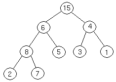
Suppose we have a complete binary tree somewhere whose subtrees are heaps. In the following complete binary tree, the subtrees of 6 are heaps:

The Heapify procedure alters the heap so that the tree rooted at 6's position is a heap. Here's how it works. First, we look at the root of our tree and its two children.

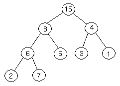
We then determine which of the three nodes is the greatest. If it is the root, we are done, because we have a heap. If not, we exchange the appropriate childwith the root, and continue recursively down the tree. In this case, we exchange 6 and 8, and continue.

Now, 7 is greater than 6, so we exchange them.
We are at the bottom of the tree, and can't continue, so we terminate.
QuickSort
There are many different versions of quickSort that pick pivot in different ways.
1) Always pick first element as pivot.
2) Always pick last element as pivot (implemented below)
3) Pick a random element as pivot.
4) Pick median as pivot.
/* This function takes last element as pivot, places the pivot element at its
   correct position in sorted array, and places all smaller (smaller than pivot)
   to left of pivot and all greater elements to right of pivot */
int partition (int arr[], int l, int h)
{
    int x = arr[h];    // pivot
    int i = (l - 1);  // Index of smaller element

    for (int j = l; j <= h- 1; j++)
    {
        // If current element is smaller than or equal to pivot
        if (arr[j] <= x)
        {
            i++;    // increment index of smaller element
            swap(&arr[i], &arr[j]);  // Swap current element with index
        }
    }
    swap(&arr[i + 1], &arr[h]);
    return (i + 1);
}

/* arr[] --> Array to be sorted, l  --> Starting index, h  --> Ending index */
void quickSort(int arr[], int l, int h)
{
    if (l < h)
    {
        int p = partition(arr, l, h); /* Partitioning index */
        quickSort(arr, l, p - 1);
        quickSort(arr, p + 1, h);
    }
}


