Merging sorted arrays in parallel and in place can be done very efficiently, using this algorithm. Comparisons with the performance of similar STL functions are included.
Introduction
In my article on parallel merge I developed and optimized a generic parallel merge algorithm. It utilized multiple CPU cores and scaled well in performance. The algorithm was stable, leading directly to Parallel Merge Sort. However, it was not an in-place implementation. In this article, I develop an in-place parallel merge, which enables in-place parallel merge sort.
The STL implements sequential merge and in-place merge algorithms, as merge() andinplace_merge(), which run on a single CPU core. The merge algorithm is O(n), leading to O(nlgn) merge sort, while the in-place merge is O(nlgn), leading to O(n(lgn)2) in-place merge sort. Because merge is faster than in-place merge, but requires extra memory, STL favors using merge whenever memory is available, copying the result back to the input array (under the hood).
Revisit Not-In-Place
The divide-and-conquer merge algorithm described in Parallel Merge, which is not-in-place, is illustrated in Figure 1. At each step, this algorithm moves a single element X from the source array T to the destination array A, as follows.

Figure 1. A merge algorithm that is not in place.
The two input sub-arrays of T are from [p1 to r1] and from [p2 to r2]. The output is a single sub-array of A from [p3 to r3]. The divide step is done by choosing the middle element within the larger of the two input sub-arrays—at index q1. The value at this index is then used as the partition element to split the other input sub-array into two sections - less than X and greater than or equal to X. The partition value X (at index q1 of T) is copied to array A at index q3. The conquer step recursively merges the two portions that are smaller than or equal to X— indicated by light gray boxes and light arrows. It also recursively merges the two portions that are larger than or equal to X—indicated by darker gray boxes and dark arrows.
The algorithm proceeds recursively until the termination condition —when the shortest of the two input sub-arrays has no elements. At each step, the algorithm reduces the size of the array by one element. One merge is split into two smaller merges, with the output element placed in between. Each of the two smaller merges will contain at least N/4 elements, since the left input array is split in half.
This algorithm is O(n) and is stable. It was shown not to be performance competitive in its pure form. However, performance became equivalent to other merges in a hybrid form, which utilized a simple merge to terminate recursion early. The hybrid version enabled parallelism by using of divide-and-conquer method, scaled well across multiple cores, outperforming STL merge by over 5X on quad-core CPU, being limited by memory bandwidth. It was also used as the core of Parallel Merge Sort, which scaled well across multiple cores, utilizing a further hybrid approach to gain more speed, and providing a high degree of parallelism, Θ(n/lg2n).
In-Place
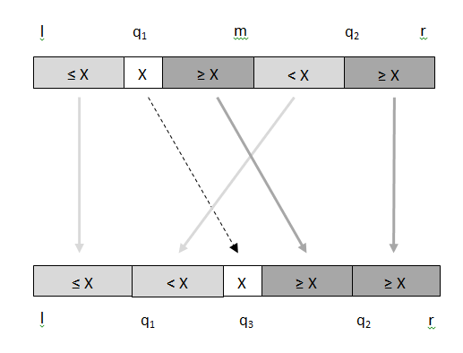
The main idea for in-place merge, illustrated in Figure 2, is based on a modification to the not-in-place merge. Instead of moving a single element X at location q1 to location q3 at each recursive step, all elements between q1 and q2 are moved using In-Place Block Swap (Block Exchange). Let's go through this in detail.

Figure 2 An in-place merge.
The top row of Figure 2 shows the input array of elements and three indexes: l, m, and r. The left segment, which is between indexes l and m, inclusive, is pre-sorted. The right segment, which is between indexes m+1 and r, inclusive, is also pre-sorted. Merge algorithm uses these two segments to produce a single sorted result. In-place merge places the result back in the input array between indexes l and r (the bottom row of Figure 1), while using a small constant amount of extra memory. Note that the two input segments touch, whereas the not-in-place merge algorithm had array elements in between the two input segments.
The first step of this divide-and-conquer algorithm is to take the larger of the two input segments, divide it in half to determine the index q1 and its value X. Then a binary search is used within the other segment to determine the index q2, at which all elements to the left are smaller than X, and all elements to the right are larger or equal to X. Thus, each of the two segments have been split into two halves, one less than X and the other greater than or equal to X. These two steps are the same as in not-in-place merge algorithm. The algorithm preserves stability because only the elements that are strictly less than X, but were to the right of X are moved to the left of X.
The next step is to in-place swap the segment q1 to m, inclusive, and the segment m+1 to q2inclusive, as shown by the diagonal arrows in Figure 2. This swap would be simple if the segments were of equal size, but this occurs rarely. In-Place Block Swap comes to the rescue, because it's capable of swapping two segments of unequal size, which are touching, in-place. Three algorithms are described in In-Place Block Swap, and the one with the highest performance along with the best parallel scaling needs to be chosen.
The algorithm proceeds recursively by processing (l, q1-1, q3-1) segment and (q3+1, q2-1, r) segments of the bottom row of Figure 1. Note that the array element X at q3 is in its final location and needs no further processing.
Sequential
Listing One shows a sequential divide-and-conquer In-Place Merge algorithm implementation. Lengths of the left and the right input array segments are computed first, determining which segment is larger. When the left (length1) segment is larger, the index of the mid-element is computed (q1). Binary search is used to split the smaller segment (m+1 to r, with length2) using the value of q1, into elements that are strictly smaller than the element at q1 (X in Figure 1). Being strictly less than X at q1, preserves stability. This binary search produces q2, which is the index of the split of the smaller segment (left segment, length2).
template< class _Type >
inline int my_binary_search( _Type value, const _Type* a, int left, int right )
{
    long low  = left;
    long high = __max( left, right + 1 );
    while( low < high )
    {
        long mid = ( low + high ) / 2;
        if ( value <= a[ mid ] ) high = mid;
        else                        low  = mid + 1; // because we compared to a[mid] and the value was larger than a[mid].
                                                    // Thus, the next array element to the right from mid is the next possible
                                                    // candidate for low, and a[mid] can not possibly be that candidate.
    }
    return high;
}
// Swaps two sequential sub-arrays ranges a[ l .. m ] and a[ m + 1 .. r ]
template< class _Type >
inline void block_exchange_mirror( _Type* a, int l, int m, int r )
{
    mirror_ptr( a, l,     m );
    mirror_ptr( a, m + 1, r );
    mirror_ptr( a, l,     r );
}
// Merge two ranges of source array T[ l .. m, m+1 .. r ] in-place.
// Based on not-in-place algorithm in 3rd ed. of "Introduction to Algorithms" p. 798-802
template< class _Type >
inline void merge_in_place_L1( _Type* t, int l, int m, int r )
{
    int length1 = m - l + 1;
    int length2 = r - m;
    if ( length1 >= length2 )
    {
        if ( length2 <= 0 )  return;                         // if the smaller segment has zero elements, then nothing to merge.
        int q1 = ( l + m ) / 2;                             // q1 is mid-point of the larger segment. length1 >= length2 > 0
        int q2 = my_binary_search( t[ q1 ], t, m + 1, r );  // q2 is q1 partitioning element within the smaller sub-array (and q2 itself is part of the sub-array that does not move)
        int q3 = q1 + ( q2 - m - 1 );
        block_exchange_mirror( t, q1, m, q2 - 1 );
        merge_in_place_L1( t, l,      q1 - 1, q3 - 1 );     // note that q3 is now in its final place and no longer participates in further processing
        merge_in_place_L1( t, q3 + 1, q2 - 1, r      );
    }
    else {  // length1 < length2
        if ( length1 <= 0 )  return;                         // if the smaller segment has zero elements, then nothing to merge
        int q1 = ( m + 1 + r ) / 2;                         // q1 is mid-point of the larger segment.  length2 > length1 > 0
        int q2 = my_binary_search( t[ q1 ], t, l, m );      // q2 is q1 partitioning element within the smaller sub-array (and q2 itself is part of the sub-array that does not move)
        int q3 = q2 + ( q1 - m - 1 );
        block_exchange_mirror( t, q2, m, q1 );
        merge_in_place_L1( t, l,      q2 - 1, q3 - 1 );     // note that q3 is now in its final place and no longer participates in further processing
        merge_in_place_L1( t, q3 + 1, q1,     r      );
    }
}
Now, that the split has been found, block swap can be performed, in-place. This moves all elements less than X to the left of X, and all element greater than or equal to X to the right of X. However, elements left of X are in two segments that now need to be merged. Also the two segments of elements right of X also need to be merged. The two recursive calls take care of these two merge operations. The else portion takes care of the opposite case—when the left segment is larger than the right segment.
Note that the in-place merge algorithm used a non-optimized non-hybrid block swap algorithm, for simplicity. An optimized hybrid algorithm is definitely a performance boosting opportunity.
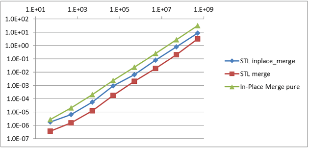
Performance of several in-place and not-in-place merge algorithms is shown in Table 1 and in Graph 1.
| Time per Run |
| Number of items |
50 |
500 |
5000 |
50000 |
500000 |
5.0E+06 |
5.0E+07 |
5.0E+08 |
| STL inplace_merge |
1.9E-06 |
6.6E-06 |
5.8E-05 |
9.1E-04 |
6.8E-03 |
8.2E-02 |
8.1E-01 |
8.8E+00 |
| STL merge |
3.6E-07 |
1.5E-06 |
1.2E-05 |
1.8E-04 |
2.0E-03 |
2.0E-02 |
2.0E-01 |
3.1E+00 |
| In-Place Merge pure |
2.9E-06 |
2.1E-05 |
2.1E-04 |
2.4E-03 |
2.4E-02 |
2.5E-01 |
2.8E+00 |
3.1E+01 |
| STL inplace_merge /
STL merge |
5.1 |
4.3 |
4.8 |
5.0 |
3.3 |
4.2 |
4.0 |
2.8 |
| In-Place Merge pure /
STL inplace_merge |
1.5 |
3.2 |
3.6 |
2.6 |
3.5 |
3.1 |
3.4 |
3.6 |
Table 1

Graph 1
STL merge is more than 2.8x faster than STL inplace_merge for all array sizes. The pure divide-and-conquer merge is more than 3X slower than STL inplace_merge for large arrays. This performance disparity may be attributed to STL inplace_merge being an adaptive algorithm, switching to STL merge when additional memory is available to allocate a temporary intermediate buffer and copying the result back to the input array. Also, nearly every algorithm that has been explored so far has performed poorly in its pure form. So, let's develop a hybrid in-place merge.
Listing Two shows such a hybrid in-place merge algorithm. STL inplace_merge is used as the recursion termination case—processing small sub-arrays.
template< class _Type >
inline void merge_in_place_1( _Type* t, int l, int m, int r )
{
    int length1 = m - l + 1;
    int length2 = r - m;
    if ( length1 >= length2 )
    {
        if ( length2 <= 0 )  return;
        if (( length1 + length2 ) <= 8192 )  { std::inplace_merge( t + l, t + m + 1, t + r + 1 );  return; }
        int q1 = ( l + m ) / 2;                             // q1 is mid-point of the larger segment
        int q2 = my_binary_search( t[ q1 ], t, m + 1, r );  // q2 is q1 partitioning element within the smaller sub-array (and q2 itself is part of the sub-array that does not move)
        int q3 = q1 + ( q2 - m - 1 );
        block_exchange_mirror( t, q1, m, q2 - 1 );      // 2X speedup
        merge_in_place_1( t, l,      q1 - 1, q3 - 1 );  // note that q3 is now in its final place and no longer participates in further processing
        merge_in_place_1( t, q3 + 1, q2 - 1, r      );
    }
    else {
        if ( length1 <= 0 )  return;
        if (( length1 + length2 ) <= 8192 )  { std::inplace_merge( t + l, t + m + 1, t + r + 1 );  return; }
        int q1 = ( m + 1 + r ) / 2;                         // q1 is mid-point of the larger segment
        int q2 = my_binary_search( t[ q1 ], t, l, m );      // q2 is q1 partitioning element within the smaller sub-array (and q2 itself is part of the sub-array that does not move)
        int q3 = q2 + ( q1 - m - 1 );
        block_exchange_mirror( t, q2, m, q1 );          // 2X speedup
        merge_in_place_1( t, l,      q2 - 1, q3 - 1 );  // note that q3 is now in its final place and no longer participates in further processing
        merge_in_place_1( t, q3 + 1, q1,     r      );
    }
}
Listing Two
Performance of the hybrid algorithm is shown in Table 2.
| Time per Run |
| Number of items |
50 |
500 |
5000 |
50000 |
500000 |
5.0E+06 |
5.0E+07 |
5.0E+08 |
| STL inplace_merge |
1.9E-06 |
6.6E-06 |
5.8E-05 |
9.1E-04 |
6.8E-03 |
8.2E-02 |
8.1E-01 |
8.8E+00 |
| In-Place Merge pure |
2.9E-06 |
2.1E-05 |
2.1E-04 |
2.4E-03 |
2.4E-02 |
2.5E-01 |
2.8E+00 |
3.1E+01 |
| In-Place Merge hybrid |
2.8E-06 |
7.0E-06 |
8.1E-05 |
9.9E-04 |
1.3E-02 |
1.6E-01 |
1.8E+00 |
1.9E+01 |
| In-Place Merge hybrid /
STL inplace_merge |
1.5 |
1.1 |
1.4 |
1.1 |
1.9 |
1.9 |
2.2 |
2.2 |
| In-Place pure /
In-Place hybrid |
1.0 |
3.1 |
2.6 |
2.4 |
1.9 |
1.6 |
1.5 |
1.6 |
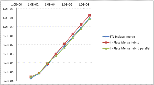
In-place hybrid merge implementation is over 1.5x faster than the pure merge, for large arrays. Interestingly, the hybrid approach for in-place merge yields less gain in performance than it did for not-in-place algorithm, where over 8.5x gain was obtained for large arrays, bringing the performance of the divide-and-conquer algorithm to nearly that of the “simple merge” (seeParallel Merge page 2, table 3). One possible reason is that in-place merge algorithm performs more memory accesses, in the block swap, becoming memory bandwidth bound instead of computationally bound. This effect is visible in Graph 2, where the performance on the hybrid algorithm starts out equal to STL inplace_merge and drifts toward in-place merge pure as the array size increases.
Graph 2
The order of the sequential divide-and-conquer in-place merge algorithm is O(nlgn), where the divide-and-conquer portion produces a tree with O(lgn) levels, with each level processing O(n) elements. The order of not-in-place merge is O(n).
Parallel
A simple, but only partially parallel algorithm falls out naturally from the implementation in Listing Two. This implementation is shown in Listing Three, where the two recursive calls have been parallelized using the parallel_invoke() of Intel TBB or Microsoft PPL. However, block swap has not yet been parallelized.
template< class _Type >
inline void p_merge_in_place_2( _Type* t, int l, int m, int r )
{
    int length1 = m - l + 1;
    int length2 = r - m;
    if ( length1 >= length2 )
    {
        if ( length2 <= 0 )  return;
        if (( length1 + length2 ) <= 1024 )  { std::inplace_merge( t + l, t + m + 1, t + r + 1 );  return; }
        int q1 = ( l + m ) / 2;                             // q1 is mid-point of the larger segment
        int q2 = my_binary_search( t[ q1 ], t, m + 1, r );  // q2 is q1 partitioning element within the smaller sub-array (and q2 itself is part of the sub-array that does not move)
        int q3 = q1 + ( q2 - m - 1 );
        block_exchange_mirror( t, q1, m, q2 - 1 );
        //tbb::parallel_invoke(
        Concurrency::parallel_invoke(
            [&] { p_merge_in_place_2( t, l,      q1 - 1, q3 - 1 ); },   // note that q3 is now in its final place and no longer participates in further processing
            [&] { p_merge_in_place_2( t, q3 + 1, q2 - 1, r      ); }
        );
    }
    else {
        if ( length1 <= 0 )  return;
        if (( length1 + length2 ) <= 1024 )  { std::inplace_merge( t + l, t + m + 1, t + r + 1 );  return; }
        int q1 = ( m + 1 + r ) / 2;                         // q1 is mid-point of the larger segment
        int q2 = my_binary_search( t[ q1 ], t, l, m );      // q2 is q1 partitioning element within the smaller sub-array (and q2 itself is part of the sub-array that does not move)
        int q3 = q2 + ( q1 - m - 1 );
        block_exchange_mirror( t, q2, m, q1 );
        //tbb::parallel_invoke(
        Concurrency::parallel_invoke(
            [&] { p_merge_in_place_2( t, l,      q2 - 1, q3 - 1 ); },   // note that q3 is now in its final place and no longer participates in further processing
            [&] { p_merge_in_place_2( t, q3 + 1, q1,     r      ); }
        );
    }
}
Listing Three
Table 3 and Graph 3 summarize performance of this partially parallel implementation.
| Time per Run |
| Number of items |
50 |
500 |
5000 |
50000 |
500000 |
5.0E+06 |
5.0E+07 |
5.0E+08 |
| STL inplace_merge |
1.9E-06 |
6.6E-06 |
5.8E-05 |
9.1E-04 |
6.8E-03 |
8.2E-02 |
8.1E-01 |
8.8E+00 |
| In-Place Merge hybrid |
2.8E-06 |
7.0E-06 |
8.1E-05 |
9.9E-04 |
1.3E-02 |
1.6E-01 |
1.8E+00 |
1.9E+01 |
| In-Place Merge hybrid parallel |
2.5E-06 |
6.9E-06 |
9.6E-05 |
5.7E-04 |
4.3E-03 |
6.0E-02 |
6.4E-01 |
8.0E+00 |
| In-Place hybrid /
In-Place parallel |
1.1 |
1.0 |
0.8 |
1.7 |
2.9 |
2.6 |
2.8 |
2.4 |
| STL inplace_merge /
In-Place parallel |
0.7 |
1.0 |
0.6 |
1.6 |
1.6 |
1.4 |
1.3 |
1.1 |
Table 3 Performance of a partially parallel implementation.

Graph 3. A graphical view of the data in Table 3.
The parallel implementation is the fastest for large arrays, running on a hyper-threaded, quad-core Intel i7-860 processor. It scaled to more than 2.4x for large array sizes over the sequential divide-and-conquer implementation, but only 10% faster than STL inplace_merge() (possibly due to the dynamic nature of STL implementation). So far, in-place merge has not scaled as well as not-in-place merge, most likely due to much higher memory bandwidth usage (in block swap, which has not been parallelized yet).
Table 4 shows how performance varies with the number of threads used to execute tasks.
| Time per Run |
| Number of items |
50 |
500 |
5000 |
50000 |
500000 |
5.0E+06 |
5.0E+07 |
5.0E+08 |
| Parallel 8 threads |
2.5E-06 |
6.9E-06 |
9.6E-05 |
5.7E-04 |
4.3E-03 |
6.0E-02 |
6.4E-01 |
8.0E+00 |
| Parallel 4 threads |
2.0E-06 |
1.7E-05 |
6.2E-05 |
4.9E-04 |
4.8E-03 |
6.3E-02 |
6.5E-01 |
8.0E+00 |
| Parallel 2 threads |
3.2E-06 |
1.1E-05 |
7.2E-05 |
5.5E-04 |
4.5E-03 |
6.1E-02 |
6.3E-01 |
8.0E+00 |
| Parallel 1 threads |
3.1E-06 |
8.2E-06 |
7.4E-05 |
6.1E-04 |
4.4E-03 |
6.3E-02 |
6.4E-01 |
7.9E+00 |
| 4 threads / 8 threads |
0.8 |
2.4 |
0.6 |
0.9 |
1.1 |
1.0 |
1.0 |
1.0 |
| 2 threads / 8 threads |
1.3 |
1.6 |
0.7 |
1.0 |
1.0 |
1.0 |
1.0 |
1.0 |
| 1 thread / 8 threads |
1.2 |
1.2 |
0.8 |
1.1 |
1.0 |
1.0 |
1.0 |
1.0 |
Table 4 How performance varies with the number of threads used to execute tasks.
Performance is nearly constant with the number of threads, which is most likely due to memory bandwidth bottleneck limiting parallel performance gain. This needs further investigation, especially because the single thread divide-and-conquer outperforms the sequential divide-and-conquer (although not by a significant amount).
Conclusion
Parallel in-place stable merge algorithm has been developed. The sequential algorithm is not new and goes back to [1], with a similar implementation in STL as inplace_merge(). The parallel implementation is an extension of Parallel Merge algorithm, using block swap/exchage algorithm to swap two inner sub-arrays of unequal size in-place. This in-place algorithm does not scale as well with the number of cores, most likely due to becoming memory bandwidth limited, yet outperforms the sequential algorithm slightly. The order of the algorithm is O(nlgn), and should extend easily into in-place stable parallel merge sort. Further performance gains could come from parallelization of block swap/exchange, along with possible elimination of redundant rotations.

