Non-Photorealistic Rendering (Domain transform for edge-aware image and video processing)
opencv 3.0 的photo模块有Non-Photorealistic Rendering 可以将进行保边的平滑滤波, 铅笔画,细节增强等等。其对应的论文是:Eduardo S. L. Gastal, Manuel M. Oliveira, “Domain transform for edge-aware image and video processing”, ACM Trans. Graph. 30(4): 69, 2011. 作者网页可以下载matlab代码
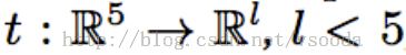
Main idea: domain transform from image in R5 (x,y,r,g,b) to lower dimension where distances are preserved. Then, perform filtering on the transformed image
在保存距离的情况下,将高维空间图像转换到低维,再对转换后图像进行滤波
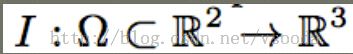
2D RGB图像I:
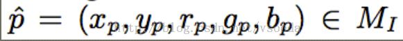
可以定义在R5上定义二维空间Mi, 令:
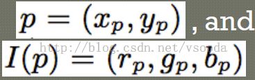
分别用空间坐标(spatial coordinates) 和值坐标(Range coordinates)表示:
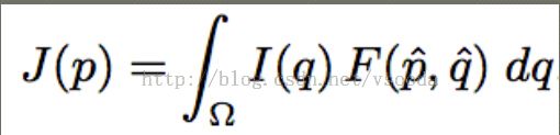
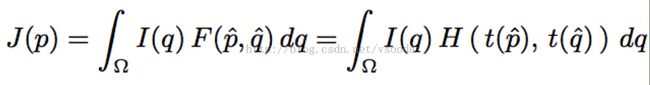
如果R5空间中的保留边滤波器为Fq, 那么滤波图像为:
需找一个转换t,使得
在Rl 上寻找一个滤波核H,其作用等同于在五维空间的滤波核F,如:
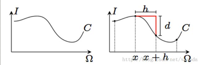
令ct(x) 表示将(x, I(x))的映射,其中(x是空间坐标,I(x)是x位置对应的r,g,b值)
转换的空间需要保存原来的距离(这里是L1),所以必须满足:
![]()
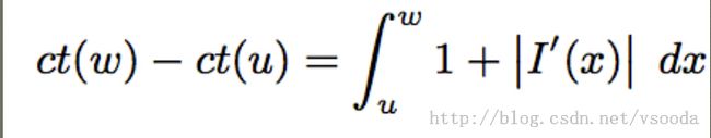
其中h是采样距离。 如下图所示,C是新的空间。线上两点的距离在距离足够小的情况下:Distance = h + d。 下面先以一维信号为例。
用积分的角度可以表示为:

在多通道的情况下,可以令导数为各通道倒数之和。

其中c是通道。
上面考虑的都是一维信号,在二维的情况下,可以对此做些扩展:1. 每一行处理; 2. 每一列处理; 3. 迭代n次
可以类似双边滤波器,将spatial和range参数都加入考虑。分别用sigma_s, sigma_r表示。
现在对图像滤波转化为:

先求解t,在选择H。H的选择至少应该比R5滤波核F更快。原文中H的选择有:Normalized Convolution, Interpolated Convolution, Recursive Filtering
文中Normalized Convolution的方法是:
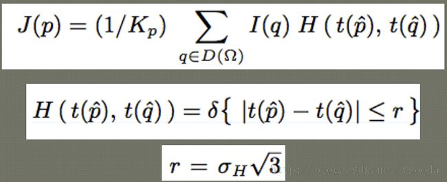
r是距离,在这个距离之内的数据进行考虑,进行插值。
文末推导了Recursive Filtering方法的参数由来,该方法实现更加简单。
opencv以该滤波方法实现了几个应用:edgePreservingFilter, detailEnhance, pencilSketch。 其中detailEnhance转化为lab,只对l分量做处理。pencilSketch转化为YCBCR进行处理
总结:
1. 作者文中提到R5到Rl, 看起来有点玄乎。后面才知道实际上是处理一维信号,对于二维先行,再列,再搞几遍。。
2. 考虑每一行,曲线上每个点的值可以看作rgb值通过某种运算等到(看代码),行上两点的距离是曲线上的距离。 现在想对某一点插值,那么就将左右距离d(曲线)内的所有点的值相加,再除以左右两点的水平距离。这样就完成了滤波。
3. 在值变化较大的区域(边缘),曲线更加陡峭,使得在相同的d内,实际上水平距离很小。这样的好处就是,在这小范围呢,像素值变化不大,更容易保留信息(边)。反之,曲线平缓,实际水平距离较大,滤波的结果会更平滑。
最后附上作者matlab程序(中文注释是我写的--):
%  NC  Domain transform normalized convolution edge-preserving filter.
%
%  F = NC(img, sigma_s, sigma_r, num_iterations, joint_image)
%
%  Parameters:
%    img             Input image to be filtered.
%    sigma_s         Filter spatial standard deviation.
%    sigma_r         Filter range standard deviation.
%    num_iterations  Number of iterations to perform (default: 3).
%    joint_image     Optional image for joint filtering.
%
%
%
%  This is the reference implementation of the domain transform NC filter
%  described in the paper:
%
%    Domain Transform for Edge-Aware Image and Video Processing
%    Eduardo S. L. Gastal  and  Manuel M. Oliveira
%    ACM Transactions on Graphics. Volume 30 (2011), Number 4.
%    Proceedings of SIGGRAPH 2011, Article 69.
%
%  Please refer to the publication above if you use this software. For an
%  up-to-date version go to:
%
%             http://inf.ufrgs.br/~eslgastal/DomainTransform/
%
%
%  THIS SOFTWARE IS PROVIDED "AS IS" WITHOUT ANY EXPRESSED OR IMPLIED WARRANTIES
%  OF ANY KIND, INCLUDING BUT NOT LIMITED TO THE WARRANTIES OF MERCHANTABILITY,
%  FITNESS FOR A PARTICULAR PURPOSE AND NONINFRINGEMENT.  IN NO EVENT SHALL THE
%  AUTHORS OR COPYRIGHT HOLDERS BE LIABLE FOR ANY CLAIM, DAMAGES OR OTHER
%  LIABILITY, WHETHER IN AN ACTION OF CONTRACT, TORT OR OTHERWISE, ARISING FROM,
%  OUT OF OR IN CONNECTION WITH THIS SOFTWARE OR THE USE OR OTHER DEALINGS IN
%  THIS SOFTWARE.
%
%  Version 1.0 - August 2011.

function F = NC(img, sigma_s, sigma_r, num_iterations, joint_image)

    I = double(img);

    if ~exist('num_iterations', 'var')
        num_iterations = 3;
    end

    if exist('joint_image', 'var') && ~isempty(joint_image)
        J = double(joint_image);

        if (size(I,1) ~= size(J,1)) || (size(I,2) ~= size(J,2))
            error('Input and joint images must have equal width and height.');
        end
    else
        J = I;
    end

    [h w num_joint_channels] = size(J);

    %% Compute the domain transform (Equation 11 of our paper). 计算公式11
    %%%%%%%%%%%%%%%%%%%%%%%%%%%%%%%%%%%%%%%%%%%%%%%%%%%%%%%%%%%%%%%%%%%%%%%%%%%%%%%%

    % Estimate horizontal and vertical partial derivatives using finite
    % differences.
    dIcdx = diff(J, 1, 2); %列差
    dIcdy = diff(J, 1, 1); %行差

    dIdx = zeros(h,w);
    dIdy = zeros(h,w);

    % Compute the l1-norm distance of neighbor pixels. dIdx 是 dIcdx的三通道绝对值之和
    for c = 1:num_joint_channels
        dIdx(:,2:end) = dIdx(:,2:end) + abs( dIcdx(:,:,c) );
        dIdy(2:end,:) = dIdy(2:end,:) + abs( dIcdy(:,:,c) );
    end

    % Compute the derivatives of the horizontal and vertical domain transforms.
    dHdx = (1 + sigma_s/sigma_r * dIdx);
    dVdy = (1 + sigma_s/sigma_r * dIdy);

    % Integrate the domain transforms.
    ct_H = cumsum(dHdx, 2);  %后面每列是前面所有列之和
    ct_V = cumsum(dVdy, 1);  %后面每行是前面所有行之和

    % The vertical pass is performed using a transposed image.
    ct_V = ct_V';

    %% Perform the filtering.
    %%%%%%%%%%%%%%%%%%%%%%%%%%%%%%%%%%%%%%%%%%%%%%%%%%%%%%%%%%%%%%%%%%%%%%%%%%%%%%%%
    N = num_iterations;
    F = I;

    sigma_H = sigma_s;

    for i = 0:num_iterations - 1

        % Compute the sigma value for this iteration (Equation 14 of our paper).
        sigma_H_i = sigma_H * sqrt(3) * 2^(N - (i + 1)) / sqrt(4^N - 1);

        % Compute the radius of the box filter with the desired variance.
        box_radius = sqrt(3) * sigma_H_i;

        F = TransformedDomainBoxFilter_Horizontal(F, ct_H, box_radius);
        F = image_transpose(F);

        F = TransformedDomainBoxFilter_Horizontal(F, ct_V, box_radius);
        F = image_transpose(F);

    end

    F = cast(F, class(img));

end

%% Box filter normalized convolution in the transformed domain.
%%%%%%%%%%%%%%%%%%%%%%%%%%%%%%%%%%%%%%%%%%%%%%%%%%%%%%%%%%%%%%%%%%%%%%%%%%%%%%%%
function F = TransformedDomainBoxFilter_Horizontal(I, xform_domain_position, box_radius)

    [h w num_channels] = size(I);

    % Compute the lower and upper limits of the box kernel in the transformed domain.
    l_pos = xform_domain_position - box_radius;
    u_pos = xform_domain_position + box_radius;

    % Find the indices of the pixels associated with the lower and upper limits
    % of the box kernel.
    %
    % This loop is much faster in a compiled language.  If you are using a
    % MATLAB version which supports the 'parallel for' construct, you can
    % improve performance by replacing the following 'for' by a 'parfor'.

    l_idx = zeros(size(xform_domain_position));
    u_idx = zeros(size(xform_domain_position));


    for row = 1:h
        %找到该行中每个元素的最左和最右位置
        xform_domain_pos_row = [xform_domain_position(row,:) inf];

        l_pos_row = l_pos(row,:);
        u_pos_row = u_pos(row,:);

        local_l_idx = zeros(1, w);
        local_u_idx = zeros(1, w);

        local_l_idx(1) = find(xform_domain_pos_row > l_pos_row(1), 1, 'first');
        local_u_idx(1) = find(xform_domain_pos_row > u_pos_row(1), 1, 'first');

        for col = 2:w
            local_l_idx(col) = local_l_idx(col-1) + ...
                find(xform_domain_pos_row(local_l_idx(col-1):end) > l_pos_row(col), 1, 'first') - 1;

            local_u_idx(col) = local_u_idx(col-1) + ...
                find(xform_domain_pos_row(local_u_idx(col-1):end) > u_pos_row(col), 1, 'first') - 1;
        end


        l_idx(row,:) = local_l_idx;
        u_idx(row,:) = local_u_idx;
    end

    % Compute the box filter using a summed area table.
    SAT            = zeros([h w+1 num_channels]);
    SAT(:,2:end,:) = cumsum(I, 2); %后面每列是前面所有列之和
    row_indices    = repmat((1:h)', 1, w);
    F              = zeros(size(I));

    for c = 1:num_channels
        %sub2ind的参数分别为size, 行, 列, channel 的矩阵
        a = sub2ind(size(SAT), row_indices, l_idx, repmat(c, h, w)); %求出每个像素空间位置对应的下标。使得最后SAT(b)就可以直接得到所有点的SAT
        b = sub2ind(size(SAT), row_indices, u_idx, repmat(c, h, w));
        F(:,:,c) = (SAT(b) - SAT(a)) ./ (u_idx - l_idx);  %SAT(b)-SAT(a)表示在radius内,像素值的积分。(u_idx-l_idx)表示实际经过的像素
    end

end

%% 多通道转置
%%%%%%%%%%%%%%%%%%%%%%%%%%%%%%%%%%%%%%%%%%%%%%%%%%%%%%%%%%%%%%%%%%%%%%%%%%%%%%%%
function T = image_transpose(I)

    [h w num_channels] = size(I);

    T = zeros([w h num_channels], class(I));

    for c = 1:num_channels
        T(:,:,c) = I(:,:,c)';
    end

end