Core Data-Structure Layer

转自：http://www.iue.tuwien.ac.at/phd/binder/node53.html

3.4Core Data-Structure Layer

This layer is responsible for

• holding the data describing the Wafer in memory and
• providing the functionality described in Section 2.2.2

The following section gives an overview of how the functionality is provided andpresents the way the various layers interact with each other in the W AFER-S TATE-S ERVER.

• 3.4.1 Required Functionality
  • 3.4.1.1 Instantiate aWafer
  • 3.4.1.2 Dump the Data
  • 3.4.1.3Point location and Interpolation
  • 3.4.1.4 Topological Operations
  • 3.4.1.5 Topographical Operations
  • 3.4.1.6 Iterators
  
  
• 3.4.2Oct-Tree
• 3.4.3Jump-and-Walk
• 3.4.4Quad-tree
• 3.4.5 Binary-Tree

3.4.1Required Functionality

The core data structures must provide methods for the following tasks:

• Instantiate a Wafer object from a persistent Wafer.
• Make the data of a Wafer object persistent.
• Provide point location and interpolation methods.
• Topological operations.
• Operations to manipulate the geometry (topography).
• Iterators over the stored data.

3.4.1.1 Instantiate aWafer

This operation is realized as one of the constructors of the Wafer class. Itexpects aReader object as argument. Data from theReader object areextracted with the algorithm depicted in Fig. 3.3.

3.4.1.2 Dump the Data

This is the inversion of the above. All data from the Wafer object are dumpedonto a file making theWafer persistent. The argument to this method is aWriter object. The algorithm that is used to dump the data is shown inFig. 3.4.

3.4.1.3Point location and Interpolation

Point location is the technique to find the surrounding grid element to a given geometrical point. Several algorithms exist to solve that problem, two of whichare offered in the WAFER-STATE-SERVER. One algorithm is tree-based and was implemented forall three dimensions (oct-tree,quad-tree, andbinary-tree). The second algorithm isbased on thejump-and-walk algorithm and is available in three dimensions. Prior toperforming an interpolation the element containing the point to interpolate mustbe determined. Thus, a local interpolation algorithm strongly depends on anefficientpoint location algorithm.

3.4.1.4 Topological Operations

Topological operations are needed to compute the interface between twosegments and to extract the boundary (hull) of theWafer. Since thesetopological data are redundant they are not stored on theWafer but computedon demand.

3.4.1.5 Topographical Operations

Topographical operations are used to modify the geometry (hull) of aWafer. The method to create a single grid (mkSingleGrid) out of a listof segments (identified by attribute names) as it is needed for device ordiffusion simulations belongs to this category. Another example is the method tomodify the Wafer geometry after an etch step (repair step).

3.4.1.6 Iterators

Iterators are access methods to query data from Wafer container objects. AWafer container is an object that holds one or more sub elements. The (top-level)Wafer object itself is such a container since it contains allobjects that comprise theWafer. All iterators in the WAFER-STATE-SERVER use the sameiteration scheme. An iterator expects a reference to an unsigned integervariable. This variable must be initialized to0 before the first call of theiterator and must not be changed afterwards. The iterator returns a handle ofthe logically next object or indicates the end of an iteration.

According to the logical contents of a persistent Wafer(Fig. 2.1) there are iterators over the points, over the segmentsand over the boundaries of aWafer.

3.4.2Oct-Tree

An oct-tree is a data structure to perform three-dimensional point locations and rangesearches. In a finiteoct-tree the geometrical data are presorted in a way thatallows efficient element searches. The space containing a grid is recursivelydecomposed into 8 sub-spaces. A sub-space can either be a node or a terminalleaf. A node is an intermediate sub-space that does not contain any elementsitself but serves as a container for other sub-nodes or sub-leafs. A terminalleaf represents a situation where a further split would not reduce the number ofelements in at least one of the resulting sub-leafs (Fig. 3.12).

The effort to search for an element in an oct-tree is of order O(log n) which gives the best possible performance among the two point location methodspresented in this thesis. This nearly optimal search performance is due to thedrastic recursive decomposition of space in 8  sub-spaces respectively. Forhomogeneous grid density, every search step reduces the remaining elements tosearch by a factor of 8.

The major disadvantages of a finite oct-tree are time consuming pre-processing and memory overheads. The pre-processing time is related to thealgorithm that inserts elements into theoct-tree. For every grid element it mustbe decided to which (already existing) sub-node it belongs. This results in alarge number of geometrical predicates that have to be computed until the finalsub-space, the so-called terminal leaf, is found. Furthermore, if a grid elementcollides with a terminal leaf, this leaf must be replaced by a node and allelements of that leaf have to be re-distributed over the newly createdsub-spaces. Depending on how the elements are shaped and how they fit intoalready existing leafs the complexity of such a test can vary significantly. Incase one of the points is contained within a leaf the test is reduced to asimple point compare operation. In the worst case the orientation of severaltetrahedrons has to be computed. Every inserted element traverses all nodesuntil it reaches the terminal leaf. On every node level all sub-spaces thatoverlap the element must be computed. For each overlapping sub-space thealgorithm recurses into the node or leaf associated to the sub-space. For ahomogeneous grid the majority of grid elements will only overlap one sub-node inany given level. Thus the amount of overlap decisions per element can beestimated to 8.D whereD is the depth of theoct-tree.

Obviously the memory overhead results from the nodes and terminal leafs that hold the data. For an average depth D of theoct-tree the number ofnodes and leafs results to:

To give an example lets compute the memory consumption including the overhead tostore a number of homogeneously distributed tetrahedrons on a32 bit machine. The average depthD is given as。According to (3.1) the number of nodes and leafs computes to. This is of the same magnitude as the number of elementsthat are stored. A tetrahedron as it is stored in theoct-tree consists of 4 point references (handles, c. f. Chapter3.7.1), thus the pertetrahedron memory consumption is 32 bytes. If we estimate an average of6tetrahedrons that share a point we have a total of pointsin our example. A point coordinate is stored as an IEEE754 double precisionfloating point number that takes8 bytes. The memory needed to store the datais then megabytes for the tetrahedrons and megabytes for the points, which gives a total of megabytes.

A node consists of 8 references to sub-nodes or leafs and tworeferences to points, which amounts to80 bytes of memory. The last of the7layers in theoct-tree structure always consists of leafs, thus the totalnumber of nodes in our example is which gives a memoryconsumption of megabytes. For the remaining leafs () the memory consumption depends on the type of the leaf. Every leaf storestwo point references. Additionally, the smallest leaf stores a reference to oneelement, the largest holds an arbitrary number of references. To make a guesswe assume that the medium number of stored element references is three. Theaverage memory consumption per leaf is then bytes and the totalamount of memory for the leafs is megabytes. The total of theintroduced memory overhead in this example amounts to104 megabytes. If werelate the memory for the data to the introduced overhead it gives. The number of overlap tests is also quite impressive, it can beestimated to be in the order of.

A finite oct-tree that implements the decomposition algorithm was developed at the Institute for Microelectronics [ 28]. The methods used to determine whether anelement overlaps a leaf are encapsulated in an interface. This allows arbitraryelements to be governed by the oct-tree as long as they implement thisinterface. Fig.  3.13 and Fig.  3.14 depict a small mesh and theresulting leaf structure in the finite oct-tree.

There is also a parallelized version of this algorithm[47,48] available that distributes sub-trees over variousnetworked computers to utilize several CPUs. For communication between thecomputers the high-level protocol CORBA [49] was used.CORBA is a standard that allows to call methods of remote objects. The location of the object is thereby transparent to the client. The connectionbetween client and remote (server) object is established via an objectreference. The references of objects are managed by the CORBA nameserver. Theclient contacts the nameserver upon startup and requests a reference to acertain object. Such a high-level protocol imposes a considerable overheadcompared to a local function call. The overhead is observed as a time delay oras a maximum number of method invocations per second. The delay is closelyrelated to speed and workload of the underlying network infrastructure.

The efficiency of the parallelization is determined by the timedelay and the remote CPU time that is consumed by the remote method. If therelation between delay and CPU time is low, or -- in other words -- if acomplex remote computation takes place, then the overhead can be neglected. Thisis the case for the fairly time consuming oct-tree insert method. During theimplementation it turned out, however, that the serialization and dynamicinstantiation of objects that is necessary to transfer an object (like, e.g. apoint) over the network is not well supported in the target language (C++)and imposes an extra programming overhead for each element type. This is in thecontrary to the design of the single-threadedoct-tree which is capable of storingarbitrary elements without the need to recompile theoct-tree source code.

Future developments will focus on a multi-threaded version of the oct-tree whereonly CPUs on one machine can be utilized.

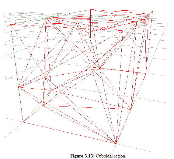
The decision whether an application uses the oct-tree or rather the jump-and-walk algorithm presented in the next section strongly depends on theamount ofpoint locations that will be performed during thesimulation. Fig. 3.13 and Fig. 3.14 show a grid of a cuboidalregion and the resulting sub-division into nodes and leafs.

3.4.3Jump-and-Walk

This technique uses a very simple algorithm to find the element surrounding agiven point. The algorithm is structured into two parts. The first part selects a start tetrahedron. The second part is an iteractive search. Beginning with the start tetrahedron, the algorithm chooses neighboring tetrahedrons such that the distance to the search point is reduced. To choose among the 4 neighboring tetrahedrons, the dot products of the normal vectors of the bounding triangles and the vector from the search to the in-sphere point of the start tetrahedronare computed. The algorithm is then repeated until either the tetrahedron containing the search point was found, or a boundary face was reached in which case the algorithm has to start at another starting tetrahedron. Fig. 3.15 depicts the principle of this algorithm.

The big advantage of this algorithm is its vanishing pre-processing time. The imposed memory overhead is also considerably smaller compared to theoct-tree. The only requirement to the data structures holding the grid elements isthat information about neighboring elements needs to be computed and held inmemory. In the following we compareoct-tree andjump-and-walk on the basis of the aboveexample (management of elements). If, for the sake ofsimplicity, the implementation of the algorithm does not distinguish betweenboundary and inner triangles, each triangle holds two handles to tetrahedronsand three point handles. We estimate the number of triangles to be, so that the total amount of memory overhead computes tomegabytes which is considerably more as with theoct-tree.

The average performance of the point location can not be estimated easily since it strongly depends on the selection of the startingelement. Several algorithms to select such an element were proposed. Onepossible strategy is to randomly choose several points (of elements) and use anelement that references the point with the smallest Euclidean distance. Anotherstrategy accounts for locations that are (possibly) geometrically related toeach other. The algorithm remembers the result of the last location and takesthis as starting condition for the next. In literature the "theoreticalperformance" forjump-and-walk on a Delaunay triangulation is given as beingproportional to (in dimensiond) when the points are randomly distributed [50].

The performance also strongly depends on the shape of thegeometry. If we look at the structure depicted in Fig. 3.16,

the thin region between the two thicker ones is unfavorable for a jump-and-walk point location algorithm in case the query point is in the thin region. Fig.  3.17 depicts a disadvantageous three-dimensional case.

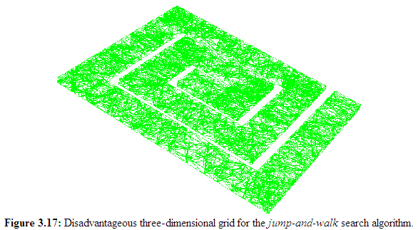
The likelihood of picking a starting element within the thicker regions isproportional to the ratio of the number of points in the two regions and thus,can be very high if the algorithm randomly chooses points and computes Euclideandistances to the query point.

Two algorithms to select a starting tetrahedron were implemented. The first algorithm uses a configurable number of randomly chosen points andpicks the one with the smallest Euclidean distance to the search point. From theset of tetrahedrons that reference this point the first is chosen as the starttetrahedron. The second selection algorithm uses apoint bucket oct-tree to store all pointsof the mesh. A point that is close to the search point is chosen. The algorithmto find a close point takes advantage of the leaf structure of thepoint bucket oct-tree inthe following manner. First the deepest node or leaf that contains at least onepoint is searched. If a leaf was found and the search point lies within thecoordinates of this leaf then the point stored on the leaf is taken as startpoint. Otherwise the neighbors of the node (or leaf) are searched. Thisalgorithm is guaranteed to return a point if thepoint bucket oct-tree is not empty. Atetrahedron is then chosen from the close point in the same way as with thefirst algorithm.

After the selection of the start tetrahedron the actual walk algorithm is started. The algorithm remembers all tetrahedrons that were already met toavoid endless loops. If the algorithm encounters the surface of the mesh,another starting tetrahedron is chosen.

The implementation of jump-and-walk is a general templatized code that supportspoint location for two-dimensional and three-dimensional grids respectively.

3.4.4Quad-tree

The quad-tree is the two-dimensional equivalent of the oct-tree. The spacecontaining the geometry is recursively decomposed into sub-spacesrespectively. As with theoct-tree the recursion stops if one of several possibleterminal situations occurs.

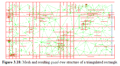
Fig. 3.18 depicts a triangulated rectangular area and the resulting leaf structure when the triangles are inserted into the tree.

3.4.5 Binary-Tree

This module is used for one-dimensional point locations. The implementation is based onanavl-tree [51]. The original implementation allows only exact pointcoordinates to be found, so the tree was extended such that linesegments can be searched.