RPL objective function & simulation using DGRM model in cooja
Introduction
The Routing Protocol for Low-Power and Lossy Networks (RPL) builds a Destination Oriented Directed Acyclic Graph (DODAG) using the Objective Function (OF). The Objective Function uses routing metrics to form the DODAG based on some algorithm or calculation formula. Basically the objective functions optimize or constrain the routing metrics that are used to form the routes and hence help in choosing the best route. There could be many objective functions in operation on the same node and mesh network because deployments vary greatly with different objectives and a single mesh network may need to carry traffic with very different requirements of path quality.
The Contiki implementation of RPL, there are 2 objective functions, but by default it uses the one that minimizes the ETX values. But the same cannot be the best routing strategy in all routing scenarios. Hence there arises a need to modify the objective function accordingly to accommodate any additional constraints or to achieve a different objective.
You Will learn
The basic assumption of this tutorial is that you know the working of the Routing Protocol for Low-Power and Lossy Networks (RPL). Here the Contiki OS 2.7v implementation of RPL is used and explained.
The following are explained in this tutorial:
- Different RPL related functions and their working
- Example scenarios and modification of RPL Objective Function
- Simulation in Cooja using DGRM model
Source Code and Directories
~/contiki-2.7/core/net/rpl/rpl-conf.h
~/contiki-2.7/core/net/rpl/rpl-of0.c
~/contiki-2.7/core/net/rpl/rpl-mrhof.c
~/contiki-2.7/tools/cooja
Related Files and Functions
Some of the important files that have the gist of RPL are rpl-config.h, rpl-of0.c, rpl-mhrof.c. However only some of the important functions in these files are mentioned here.
rpl-config.h
RPL_CONF_STATS
/* RPL_CONF_STATS */
#ifndef RPL_CONF_STATS
#define RPL_CONF_STATS 0
#endif
Here RPL Configuration statistics are disabled. To enable we need it to set to 1.
RPL_DAG_MC
/* RPL_CONF_DAG_MC */
#ifdef RPL_CONF_DAG_MC
#define RPL_DAG_MC RPL_CONF_DAG_MC
#else
#define RPL_DAG_MC RPL_DAG_MC_NONE
#endif
Here RPL metric container of the type using ETX and ENERGY are supported. However if you develop an objective function and an associated metric container can be supported.
RPL_OF
/* RPL_CONF_OF */
#ifdef RPL_CONF_OF
#define RPL_OF RPL_CONF_OF
#else
#define RPL_OF rpl_mrhof
#endif
The RPL_CONF_OF parameter configures the RPL objective function. ETX is the default objective function here. This should be defined to be the name of an rpl_of object linked into the system image, e.g., rpl_of0. Here you can also define it to be your own developed Objective function.
RPL_LEAF_ONLY
#ifdef RPL_CONF_LEAF_ONLY
#define RPL_LEAF_ONLY RPL_CONF_LEAF_ONLY
#else
#define RPL_LEAF_ONLY 0
#endif
The node should stay as a leaf node or not is decided by this value.(as mentioned in draft-ietf-roll-rpl-19#section-8.5)
RPL_INIT_LINK_METRIC
#ifndef RPL_CONF_INIT_LINK_METRIC
#define RPL_INIT_LINK_METRIC        5
#else
#define RPL_INIT_LINK_METRIC        RPL_CONF_INIT_LINK_METRIC
#endif
This is the initial metric attributed to the link when ETX is unknown. It can be changed to any desirable value. Further as we will see we will set this value to 1.
rpl-of0.c
An implementation of RPL's objective function 0 is in this file.
calculate_rank(rpl_parent_t *p, rpl_rank_t base_rank)
static rpl_rank_t
 calculate_rank(rpl_parent_t *p, rpl_rank_t base_rank)
 {
  rpl_rank_t increment;
  if(base_rank == 0) {
    if(p == NULL) {
      return INFINITE_RANK;
    }
    base_rank = p->rank;
  }

  increment = p != NULL ?
                p->dag->instance->min_hoprankinc :
                DEFAULT_RANK_INCREMENT;

  if((rpl_rank_t)(base_rank + increment) < base_rank) {
    PRINTF("RPL: OF0 rank %d incremented to infinite rank due to wrapping\n",
        base_rank);
    return INFINITE_RANK;
  }
  return base_rank + increment;
 }
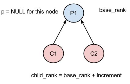
Here rank of a node is calculated. The rank of the node is based on its parents rank and base rank. If the base rank is zero and the node has no parent then the rank of the node is infinite. If the base rank is zero and parent is present then the base rank becomes equal to the parent rank. If the base rank is not zero, then depending if the parent is present or not the increment becomes min_hoprankinc of the parent in the DAG instance or DEFAULT_RANK_INCREMENT. In short if Parent is NULL then base_rank is incremented by a default increment else it uses information about parent to increment the base_rank. In the last part, if the calculated new rank is less than the base rank then the new rank becomes infinity due to wrapping around. The new calculated rank is equal to the base rank added with the increment.
best_dag(rpl_dag_t *d1, rpl_dag_t *d2)
static rpl_dag_t *
best_dag(rpl_dag_t *d1, rpl_dag_t *d2)
{
  if(d1->grounded) {
    if (!d2->grounded) {
      return d1;
    }
  } else if(d2->grounded) {
    return d2;
  }

  if(d1->preference < d2->preference) {
    return d2;
  } else {
    if(d1->preference > d2->preference) {
      return d1;
    }
  }

  if(d2->rank < d1->rank) {
    return d2;
  } else {
    return d1;
  }
}
This function compares two DAGs and returns the best of the Two DAGs (passed as input d1 and d2)according to the Objective function. There are 3 criteria to find the best DAG here. The first one is to find if the DAG is grounded. Second is the preference metric of each DAG. The third one is the rank of each DAG.
best_parent(rpl_parent_t *p1, rpl_parent_t *p2)
static rpl_parent_t *
best_parent(rpl_parent_t *p1, rpl_parent_t *p2)
{
  rpl_rank_t r1, r2;
  rpl_dag_t *dag;

  PRINTF("RPL: Comparing parent ");
  PRINT6ADDR(rpl_get_parent_ipaddr(p1));
  PRINTF(" (confidence %d, rank %d) with parent ",
        p1->link_metric, p1->rank);
  PRINT6ADDR(rpl_get_parent_ipaddr(p2));
  PRINTF(" (confidence %d, rank %d)\n",
        p2->link_metric, p2->rank);


  r1 = DAG_RANK(p1->rank, p1->dag->instance) * RPL_MIN_HOPRANKINC  +
         p1->link_metric;
  r2 = DAG_RANK(p2->rank, p1->dag->instance) * RPL_MIN_HOPRANKINC  +
         p2->link_metric;

  dag = (rpl_dag_t *)p1->dag; /* Both parents must be in the same DAG. */
  if(r1 < r2 + MIN_DIFFERENCE &&
     r1 > r2 - MIN_DIFFERENCE) {
    return dag->preferred_parent;
  } else if(r1 < r2) {
    return p1;
  } else {
    return p2;
  }
}
This function compares two parents and returns the best one according to the Objective function. Here the parents are compared based on their rank and the ETX value of that parent. This is one of the important functions, since the route formation is based on this after choosing the best DAG.
rpl-mhrof.c
The Minimum Rank with Hysteresis Objective Function (MRHOF) is implemented in this file. The objective function uses ETX as routing metric and it also has stubs for energy metric.
calculate_path_metric(rpl_parent_t *p)
static rpl_path_metric_t
calculate_path_metric(rpl_parent_t *p)
{
  if(p == NULL) {
    return MAX_PATH_COST * RPL_DAG_MC_ETX_DIVISOR;
  }

#if RPL_DAG_MC == RPL_DAG_MC_NONE
  return p->rank + (uint16_t)p->link_metric;
#elif RPL_DAG_MC == RPL_DAG_MC_ETX
  return p->mc.obj.etx + (uint16_t)p->link_metric;
#elif RPL_DAG_MC == RPL_DAG_MC_ENERGY
  return p->mc.obj.energy.energy_est + (uint16_t)p->link_metric;
#else
#error "Unsupported RPL_DAG_MC configured. See rpl.h."
#endif /* RPL_DAG_MC */
}
Here path metric is calculated according to the OF. If no parent is present then a default metric which is calculated based on Maximum Path Cost is used. If no OF is mentioned then path metric is sum of rank( and link metric. For OF based on ETX, it is sum of ETX measured (p->mc.obj.etx) and link metric. Similarly if the OF is based on Energy then energy value (p->mc.obj.energy.energy_est) is added to the link metric. This function is called by best_parent() to compare the path metrics of the two parents.
neighbor_link_callback(rpl_parent_t *p, int status, int numtx)
static void
neighbor_link_callback(rpl_parent_t *p, int status, int numtx)
{
  uint16_t recorded_etx = p->link_metric;
  uint16_t packet_etx = numtx * RPL_DAG_MC_ETX_DIVISOR;
  uint16_t new_etx;

  /* Do not penalize the ETX when collisions or transmission errors occur. */
  if(status == MAC_TX_OK || status == MAC_TX_NOACK) {
    if(status == MAC_TX_NOACK) {
      packet_etx = MAX_LINK_METRIC * RPL_DAG_MC_ETX_DIVISOR;
    }

    new_etx = ((uint32_t)recorded_etx * ETX_ALPHA +
               (uint32_t)packet_etx * (ETX_SCALE - ETX_ALPHA)) / ETX_SCALE;

    PRINTF("RPL: ETX changed from %u to %u (packet ETX = %u)\n",
        (unsigned)(recorded_etx / RPL_DAG_MC_ETX_DIVISOR),
        (unsigned)(new_etx  / RPL_DAG_MC_ETX_DIVISOR),
        (unsigned)(packet_etx / RPL_DAG_MC_ETX_DIVISOR));
    p->link_metric = new_etx;
  }
}
This function receives link-layer neighbor information. The parameter status is set either to 0 or 1. The numetx parameter specifies the current ETX(estimated transmissions) for the neighbor. The recorded ETX is the link_metric and packet ETX is the numetx parameter passed to the function. The new_etx is calculated based on the formula using both the recorded and packet ETX values. The link_metric is updated with the new ETX value.
calculate_rank(rpl_parent_t *p, rpl_rank_t base_rank)
static rpl_rank_t
calculate_rank(rpl_parent_t *p, rpl_rank_t base_rank)
{
  rpl_rank_t new_rank;
  rpl_rank_t rank_increase;

  if(p == NULL) {
    if(base_rank == 0) {
      return INFINITE_RANK;
    }
    rank_increase = RPL_INIT_LINK_METRIC * RPL_DAG_MC_ETX_DIVISOR;
  } else {
    rank_increase = p->link_metric;
    if(base_rank == 0) {
      base_rank = p->rank;
    }
  }

  if(INFINITE_RANK - base_rank < rank_increase) {
    /* Reached the maximum rank. */
    new_rank = INFINITE_RANK;
  } else {
   /* Calculate the rank based on the new rank information from DIO or
      stored otherwise. */
    new_rank = base_rank + rank_increase;
  }

  return new_rank;
}
This is similar to the calculate_rank() function explained earlier but with a slight difference. In this OF, the rank_increase is the increment which is equal toRPL_INIT_LINK_METRIC if parent = NULL. Else it is equal to the link_metric. The new rank is the increment added to the base rank.
best_parent(rpl_parent_t *p1, rpl_parent_t *p2)
static rpl_parent_t *
best_parent(rpl_parent_t *p1, rpl_parent_t *p2)
{
  rpl_dag_t *dag;
  rpl_path_metric_t min_diff;
  rpl_path_metric_t p1_metric;
  rpl_path_metric_t p2_metric;

  dag = p1->dag; /* Both parents are in the same DAG. */

  min_diff = RPL_DAG_MC_ETX_DIVISOR /
             PARENT_SWITCH_THRESHOLD_DIV;

  p1_metric = calculate_path_metric(p1);
  p2_metric = calculate_path_metric(p2);

  /* Maintain stability of the preferred parent in case of similar ranks. */
  if(p1 == dag->preferred_parent || p2 == dag->preferred_parent) {
    if(p1_metric < p2_metric + min_diff &&
       p1_metric > p2_metric - min_diff) {
      PRINTF("RPL: MRHOF hysteresis: %u <= %u <= %u\n",
             p2_metric - min_diff,
             p1_metric,
             p2_metric + min_diff);
      return dag->preferred_parent;
    }
  }

  return p1_metric < p2_metric ? p1 : p2;
}
This is similar tto the best_parent() function earlier which compares the two parents and returns the best one. Here path metric calculated for each parent is the basis for comparison. First it is checked if any of the parent is set as the preferred parent in the DAG formed and if so then it is chosen as the best parent (based on the MRHOF hysteresis RFC 6719). Otherwise, the two calculated metrics are compared and the parent with the lower metric is the best parent. In this OF, a switch is made to that minimum Rank path only if it is shorter (in terms of path cost) than the current path by at least a given threshold. This second mechanism is called "hysteresis" (RFC 6719).Here the PARENT_SWITCH_THRESHOLD_DIV is defined to be 2.
This parent selection occurs in the following cases
- during the initial formation of the network or
- when path cost to the neighboring nodes changes or
- a new node appears in the neighborhood of the node
Example scenario for objective function modification
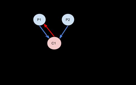
The above figure shows a sample topology which can be used.
An objective function basically uses a link metric and has function which subject to a contraint tries to choose the best path for routing. To define a completely new Objective Function file(without modifying the existing one) the following functions must be defined in them. Also the makefile should be accordingly modified and care should be taken that your new file should not run into compilation and linking errors. Some of the API for RPL Objective function are:
- reset(dag): Resets the objective function state for a specific DAG. This function is called when doing a global repair on the DAG.
- neighbor_link_callback(parent, status, etx): Receives link-layer neighbor information.
- best_parent(parent1, parent2): Compares two parents and returns the best one, according to the OF.
- best_dag(dag1, dag2): Compares two DAGs and returns the best one, according to the OF.
- calculate_rank(parent, base_rank): Calculates a rank value using the parent rank and a base rank.
- update_metric_container(dag): Updates the metric container for outgoing DIOs in a certain DAG. If the objective function of the DAG does not use metric containers, the function should set the object type to RPL_DAG_MC_NONE.
An example for modifying the objective function can be for Load Balancing application. The new objective function should be such that it should choose a route that minimizes the ETX and if there are multiple routes with same ETX or having ETX in a predefined range then it should minimize the maximum number of packets forwarded by any one of these routes. This means that any one node is not burdened with the load of forwarding packets while other nodes are under utilized.
One approach to this problem is to define a completely new objective function as described earlier. Another approach is to modify the already present rpl-mhrof.c file. As this OF already uses the minimum ETX part of the problem we just have to implement the load balancing part. The load balancing comes in to picture when a child has multiple routes i.e. parents. Hence the best parent function shouhld be modified accordingly.
Another example could be to choose the shortest path with nodes using minimum energy. Here the objective function should be such that it first identifies the nodes using minimum energy or within a range and then use minimum hops to reach the destination using these nodes. This can have an application in situation where a node has to quickly send its data without burdening a node which is deficient of energy.
In this scenario the objective function using energy metric which is already present in the current implementation of rpl-mhrof,c can be used with additional logic for choosing minimum hop count while choosing a parent.
Other scenarios which necessitate a new or modified objective function can be based on different link metrics such as throughput, link quality level, latency etc.
Cooja Simulation using DGRM model
The DGRM model is used since it is easier to change the link reception rate. Also it is easier to form a link between two desired nodes excluding the others. The following are the steps to form a new simulation:
Note: You can refer to Cooja Simulator for an introduction to Cooja.
- Run Cooja
Go to your Contiki folder(contiki-2.7) and then go to /tools/cooja directory
Run the command sudo ant run to open up a cooja GUI.
$ cd contiki-2.7/tools/cooja
$ sudo ant run
- Start a New Simulation
Choose a New Simulation from the File drop down menu (or alternatively can do Ctrl+N).
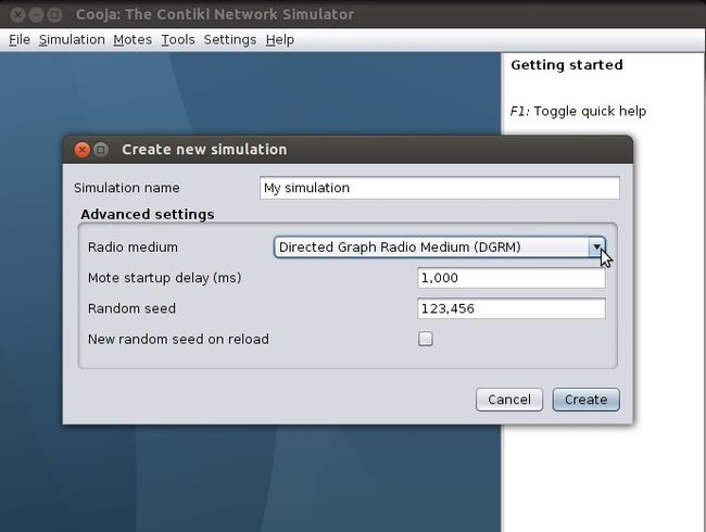
The following screen will pop up.
Give a name to your simulation in the Simulation Name field. Choose the Directed Graph Radio Medium(DGRM) from the drop down menu for the Radio Medium under Advanced Settings. Click on the Create button.
The new simulation created will open up multiple windows as shown.
- Add Sink Mote
Add a mote of the type Sink. Here udp-sink code from the rpl-collect example (/examples/ipv6/rpl-collect/) is being used. However you can upload any code you want to implement according to your application. Click on Compile button. A Create button will appear on successful compilation which adds number of motes as desired in the network. Here only one sink is used.
- Add Sender Motes
Add a mote of the type Sink. Here udp-sender code from the rpl-collect example (/examples/ipv6/rpl-collect/) is being used. However you can upload any code you want to implement according to your application.
Compile the code and create many motes of this type according to the topology.
Note: Placement of the mote does not matter here. You can place your motes anywhere in the graph. Since this is different than the distance model, we make explicit links between the motes for communication, hence distance between them makes no difference.
- Add Communication Links
Add two communication links between each set of nodes so that the communication can be bidirectional.
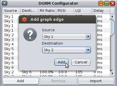
Click on Tools->DGRM Links... This will open a DGRM Configurator Dialog box. Click on Add. Select source and destination nodes and again click on add. This will add a unidirectional link from the source to destination node. For a bidirectional link you need to add one more link with source and destination nodes switched. You can add multiple links in this way. After adding the links close the dialog box.
You can change other parameters of the link such as RX ratio, RSSI, LQI and Delay according to your application. These parameters affect the individual link quality eg. RX ratio affect the ETX values. So to test your application under various Link Quality conditions these parameters can be changed.
Also you can Delete an existing one using the remove option. The Import option helps in importing any data file which already has these link connections and parameters specified in it.
- Run Simulation
Run the simulation by using the Start option in the Simulation Control window. This will initiate the motes and allocate all with a new Rime address and other initialization processes.
- Watch Output
The motes output and debug messages can be seen in the Motes Output window. You can filter the output based on the node ID:node_id to watch a particular node. You can also watch particular debug messages by filtering them. The other useful functions of the Motes Output are File, Edit and View. The File option helps in saving the output to a file. The Edit has the option of copying the output - either full or a particular selected messages. You can also clear the messages using the Clear all messages option.
You can use these messages saved in file to make observations and plot graphs according to the objective of your experiment.
General Issues
While running cooja be sure to run as sudo ant run since running only ant run might throw up some errors since it might not be able to access some files.
If the network is huge or ETX values are large, it might take a while for the packets from the leaf node to reach the root sink node. Hence you might have to run the simulation for a long time.
References
RFC 6550 RPL: IPv6 Routing Protocol for Low-Power and Lossy Networks
RFC 6552 Objective Function Zero for the Routing Protocol for Low-Power and Lossy Networks (RPL)
RFC 6719 MRHOF: The Minimum Rank with Hysteresis Objective Function
[1] IPSO Alliance RPL April 2011
[2] ContikiRPL
https://github.com/contiki-os/contiki/tree/release-2-7 Github branch of ContikiOS-2.7
Edited by - Ashwini Telang


