Correlation

The correlation is one of the most common and most useful statistics. A correlation is a single number that describes the degree of relationship between two variables. Let's work through an example to show you how this statistic is computed.

Correlation Example

Let's assume that we want to look at the relationship between two variables, height (in inches) and self esteem. Perhaps we have a hypothesis that how tall you are effects your self esteem (incidentally, I don't think we have to worry about the direction of causality here -- it's not likely that self esteem causes your height!). Let's say we collect some information on twenty individuals (all male -- we know that the average height differs for males and females so, to keep this example simple we'll just use males). Height is measured in inches. Self esteem is measured based on the average of 10 1-to-5 rating items (where higher scores mean higher self esteem). Here's the data for the 20 cases (don't take this too seriously -- I made this data up to illustrate what a correlation is):

Person	Height	Self Esteem
1	68	4.1
2	71	4.6
3	62	3.8
4	75	4.4
5	58	3.2
6	60	3.1
7	67	3.8
8	68	4.1
9	71	4.3
10	69	3.7
11	68	3.5
12	67	3.2
13	63	3.7
14	62	3.3
15	60	3.4
16	63	4.0
17	65	4.1
18	67	3.8
19	63	3.4
20	61	3.6

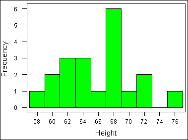
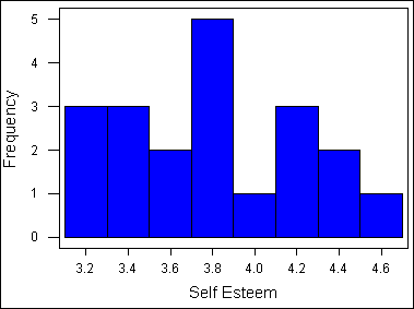
Now, let's take a quick look at the histogram for each variable:

And, here are the descriptive statistics:

Variable	Mean	StDev	Variance	Sum	Minimum	Maximum	Range
Height	65.4	4.40574	19.4105	1308	58	75	17
Self Esteem	3.755	0.426090	0.181553	75.1	3.1	4.6	1.5

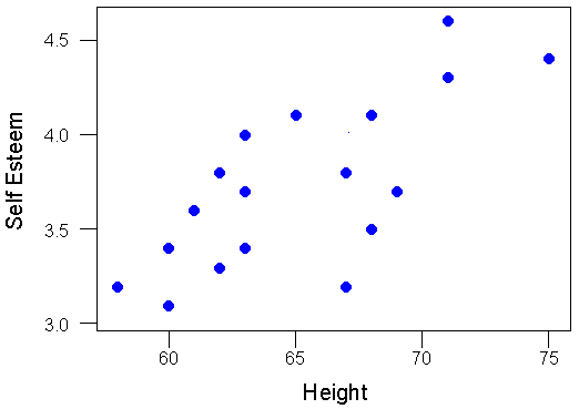
Finally, we'll look at the simple bivariate (i.e., two-variable) plot:

You should immediately see in the bivariate plot that the relationship between the variables is a positive one (if you can't see that, review the section on types of relationships) because if you were to fit a single straight line through the dots it would have a positive slope or move up from left to right. Since the correlation is nothing more than a quantitative estimate of the relationship, we would expect a positive correlation.

What does a "positive relationship" mean in this context? It means that, in general, higher scores on one variable tend to be paired with higher scores on the other and that lower scores on one variable tend to be paired with lower scores on the other. You should confirm visually that this is generally true in the plot above.

Calculating the Correlation

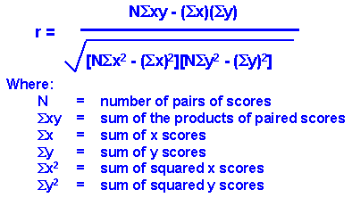
Now we're ready to compute the correlation value. The formula for the correlation is:

We use the symbol r to stand for the correlation. Through the magic of mathematics it turns out that r will always be between -1.0 and +1.0. if the correlation is negative, we have a negative relationship; if it's positive, the relationship is positive. You don't need to know how we came up with this formula unless you want to be a statistician. But you probably will need to know how the formula relates to real data -- how you can use the formula to compute the correlation. Let's look at the data we need for the formula. Here's the original data with the other necessary columns:

Person	Height (x)	Self Esteem (y)	x*y	x*x	y*y
1	68	4.1	278.8	4624	16.81
2	71	4.6	326.6	5041	21.16
3	62	3.8	235.6	3844	14.44
4	75	4.4	330	5625	19.36
5	58	3.2	185.6	3364	10.24
6	60	3.1	186	3600	9.61
7	67	3.8	254.6	4489	14.44
8	68	4.1	278.8	4624	16.81
9	71	4.3	305.3	5041	18.49
10	69	3.7	255.3	4761	13.69
11	68	3.5	238	4624	12.25
12	67	3.2	214.4	4489	10.24
13	63	3.7	233.1	3969	13.69
14	62	3.3	204.6	3844	10.89
15	60	3.4	204	3600	11.56
16	63	4	252	3969	16
17	65	4.1	266.5	4225	16.81
18	67	3.8	254.6	4489	14.44
19	63	3.4	214.2	3969	11.56
20	61	3.6	219.6	3721	12.96
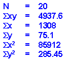
Sum =	1308	75.1	4937.6	85912	285.45

The first three columns are the same as in the table above. The next three columns are simple computations based on the height and self esteem data. The bottom row consists of the sum of each column. This is all the information we need to compute the correlation. Here are the values from the bottom row of the table (where N is 20 people) as they are related to the symbols in the formula:

Now, when we plug these values into the formula given above, we get the following (I show it here tediously, one step at a time):

So, the correlation for our twenty cases is .73, which is a fairly strong positive relationship. I guess there is a relationship between height and self esteem, at least in this made up data!

Testing the Significance of a Correlation

Once you've computed a correlation, you can determine the probability that the observed correlation occurred by chance. That is, you can conduct a significance test. Most often you are interested in determining the probability that the correlation is a real one and not a chance occurrence. In this case, you are testing the mutually exclusive hypotheses:

Null Hypothesis:	r = 0
Alternative Hypothesis:	r <> 0

The easiest way to test this hypothesis is to find a statistics book that has a table of critical values of r. Most introductory statistics texts would have a table like this. As in all hypothesis testing, you need to first determine the significance level. Here, I'll use the common significance level of alpha = .05. This means that I am conducting a test where the odds that the correlation is a chance occurrence is no more than 5 out of 100. Before I look up the critical value in a table I also have to compute the degrees of freedom or df. The df is simply equal to N-2 or, in this example, is 20-2 = 18. Finally, I have to decide whether I am doing a one-tailedor two-tailed test. In this example, since I have no strong prior theory to suggest whether the relationship between height and self esteem would be positive or negative, I'll opt for the two-tailed test. With these three pieces of information -- the significance level (alpha = .05)), degrees of freedom (df = 18), and type of test (two-tailed) -- I can now test the significance of the correlation I found. When I look up this value in the handy little table at the back of my statistics book I find that the critical value is .4438. This means that if my correlation is greater than .4438 or less than -.4438 (remember, this is a two-tailed test) I can conclude that the odds are less than 5 out of 100 that this is a chance occurrence. Since my correlation 0f .73 is actually quite a bit higher, I conclude that it is not a chance finding and that the correlation is "statistically significant" (given the parameters of the test). I can reject the null hypothesis and accept the alternative.

The Correlation Matrix

All I've shown you so far is how to compute a correlation between two variables. In most studies we have considerably more than two variables. Let's say we have a study with 10 interval-level variables and we want to estimate the relationships among all of them (i.e., between all possible pairs of variables). In this instance, we have 45 unique correlations to estimate (more later on how I knew that!). We could do the above computations 45 times to obtain the correlations. Or we could use just about any statistics program to automatically compute all 45 with a simple click of the mouse.

I used a simple statistics program to generate random data for 10 variables with 20 cases (i.e., persons) for each variable. Then, I told the program to compute the correlations among these variables. Here's the result:

          C1       C2       C3       C4       C5       C6       C7       C8       C9      C10
C1     1.000 C2     0.274    1.000
C3    -0.134   -0.269    1.000
C4     0.201   -0.153    0.075    1.000
C5    -0.129   -0.166    0.278   -0.011    1.000
C6    -0.095    0.280   -0.348   -0.378   -0.009    1.000
C7     0.171   -0.122    0.288    0.086    0.193    0.002    1.000
C8     0.219    0.242   -0.380   -0.227   -0.551    0.324   -0.082    1.000
C9     0.518    0.238    0.002    0.082   -0.015    0.304    0.347   -0.013    1.000
C10    0.299    0.568    0.165   -0.122   -0.106   -0.169    0.243    0.014    0.352    1.000

This type of table is called a correlation matrix. It lists the variable names (C1-C10) down the first column and across the first row. The diagonal of a correlation matrix (i.e., the numbers that go from the upper left corner to the lower right) always consists of ones. That's because these are the correlations between each variable and itself (and a variable is always perfectly correlated with itself). This statistical program only shows the lower triangle of the correlation matrix. In every correlation matrix there are two triangles that are the values below and to the left of the diagonal (lower triangle) and above and to the right of the diagonal (upper triangle). There is no reason to print both triangles because the two triangles of a correlation matrix are always mirror images of each other (the correlation of variable x with variable y is always equal to the correlation of variable y with variable x). When a matrix has this mirror-image quality above and below the diagonal we refer to it as asymmetric matrix. A correlation matrix is always a symmetric matrix.

To locate the correlation for any pair of variables, find the value in the table for the row and column intersection for those two variables. For instance, to find the correlation between variables C5 and C2, I look for where row C2 and column C5 is (in this case it's blank because it falls in the upper triangle area) and where row C5 and column C2 is and, in the second case, I find that the correlation is -.166.

OK, so how did I know that there are 45 unique correlations when we have 10 variables? There's a handy simple little formula that tells how many pairs (e.g., correlations) there are for any number of variables:

where N is the number of variables. In the example, I had 10 variables, so I know I have (10 * 9)/2 = 90/2 = 45 pairs.

Other Correlations

The specific type of correlation I've illustrated here is known as the Pearson Product Moment Correlation. It is appropriate when both variables are measured at an interval level. However there are a wide variety of other types of correlations for other circumstances. for instance, if you have two ordinal variables, you could use the Spearman rank Order Correlation (rho) or the Kendall rank order Correlation (tau). When one measure is a continuous interval level one and the other is dichotomous (i.e., two-category) you can use the Point-Biserial Correlation. For other situations, consulting the web-based statistics selection program, Selecting Statisticsat http://trochim.human.cornell.edu/selstat/ssstart.htm.

http://www.socialresearchmethods.net/kb/statcorr.php