REAL-TIME 3D RECONSTRUCTION USING SIGNED DISTANCE FUNCTIONS
http://www.personal.psu.edu/users/j/p/jpm5375/assignment6.html/
John Morgan
Motivation
With the recent influx of inexpensive depth sensors such as the Microsoft Kinect, systems for 3D reconstruction and visual odometry utilizing depth have garnered new interest. The combination of these two tasks is known as simultaneous localization and mapping (SLAM). Localization refers to the estimation of the camera pose and mapping refers to the amalgamation of all measurements into a single, global model. Additionally, through the use of parallel hardware it is possible to utilize all available data in real-time.
This is of particular interest for robotic navigation and interactive virtual reality, though there are countless other applications. Google is already pioneering SLAM systems on mobile devices with Project Tango. Imagine going beyond photos and creating 3D digital reconstructions in mere seconds, or being able to place and interact with virtual objects as if they were really there by simply scanning the room with your phone. The possibilities are truly exciting, but they are still out of reach.
Recent work has shown that representing the global model as a truncated signed distance function (TSDF) offers many computational advantages over the explicit storage of 3D points. The representation of choice is that proposed by Curless and Levoy [1], and the recent Kinect Fusion algorithm by Newcombe et al. [2] demonstrates real-time capability when parallel hardware is available. However, the usefulness of TSDFs extends beyond mere volumetric representation. Kubacki [3] and Canelhas [4] both present methods for carrying out pose estimation through direct use of the TSDF.
The Truncated Signed Distance Function
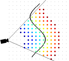
A TSDF is an arbitrary grid of points in space, referred to as voxels, which contain the distance to the nearest surface. Because surfaces should only influence a nearby region, the distance is cut off at some truncation distance beyond which becomes empty space. This is a special case of the level set method that has a gradient magnitude of 1 at all non-empty, continuous points.
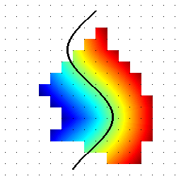
The surface itself is implicitly defined where the distance is zero. To make this easy to detect, distances in front of the surface are positive and distances behind the surface (inside the object) are negative. By doing this one needs only to find the point where the distance changes sign to locate the surface.
This is easy to visualize in 2D. In the image below the black line is an observed surface and the distance is represented by color: the zero crossing is green, positive distances are blue to green, and negative distances are green to red
To resolve distances between voxels, linear interpolation can be used. This yields a continuous function from the discrete representation
In addition to having a magnitude of 1, the gradient of this function at any point is perpendicular to the nearest surface. This means the gradient at a surface is the surface normal. Surface normals are very important for virtual reality because they determine how one object interacts with another. While a gradient can be found with a simple finite difference, finding the normal using a set of 3D points would require nearest neighbor searching and Eigen decomposition.
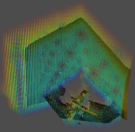
Below is a real-world example of a TSDF
Advantages as a Global Model
There are many desirable features for the global model, some of the most important include:
Incorporation of all measurements, including redundant onesThe best models are those that can utilize all the available data. However, there will always be some error associated with the sensor. By taking advantage of redundant measurements this error can be reduced.
Ability to be incrementally updated
New data needs to be incorporated into the model as it is obtained. For a TSDF this is as simple as maintaining a running average for the distance at each voxel
Where D and W are the cumulative distances and weights and d and w are the current distances and weights. Each voxel can be considered individually, so TSDFs are an excellent fit for parallel hardware.
Speed and storage
While there are many speedups associated with TSDFs, it is all at the expense of memory. Maintaining a three-dimensional array of voxel distances can quickly become unmanageable for large or high resolution volumes.
Advantages for Pose Estimation
One of the most commonly used methods for registering sets of points is the iterative closest point (ICP) algorithm. In order to run ICP the points in each cloud must be matched, which is not a trivial task. The simplest solution is to pair each point p with its nearest neighbor q in the other set then minimize the sum of squared distances
While there are closed form solutions to this equation, nearest neighbor searching is computationally expensive and difficult to parallelize.
Recall that the gradients of the TSDF point towards the nearest surface and the distances encode how far away the surface is. Kubacki [3] takes advantage of these properties by matching points with their projections onto the nearest surface, obtained by progressing the points along the gradient by the TSDF distance. This is much easier than nearest neighbor searching and aligns points to a continuous surface rather than another set of points. This is not the only solution, for example Canelhas [4] takes an entirely different approach.
References
- R.A. Newcombe, S. Izadi, O. Hilliges, D. Molyneaux, D. Kim, A.J. Davison, P. Kohli, J. Shotton, S. Hodges, and A.W. Fitzgibbon. KinectFusion: Real-time dense surface mapping and tracking. In ISMAR, pages 127–136, 2011.
- B. Curless and M. Levoy. A volumetric method for building complex models from range images. In SIGGRAPH, 1996.
- Daniel B. Kubacki; Huy Q. Bui; S. Derin Babacan and Minh N. Do "Registration and integration of multiple depth images using signed distance function", Proc. SPIE 8296, Computational Imaging X, 82960Z (February 9, 2012)
- D. RICAO CANELHAS, “Scene representation, registration and object detection in a truncated signed distance function representation of 3d space,” Master’s thesis, Örebro University, 2012.


