Theano-Deep Learning Tutorials 笔记:Restricted Boltzmann Machines
教程地址:http://www.deeplearning.net/tutorial/rbm.html
强烈建议!烈建议!强烈建议:看受限波尔兹曼机一定要看的博客,详细得当场就跪下了,博客后面的参考文献也很值得一读,互相对比理解:http://blog.csdn.net/itplus/article/details/19168937
有时间也得好好学学概率图模型
Energy-Based Models (EBM)
这段话不太好翻译过来,只知道大概啥意思。
Energy-based models associate a scalar energy to each configuration of the variables of interest. Learning corresponds to modifying that energy function so that its shape has desirable properties. For example, we would like plausible or desirable configurations to have low energy.
Energy-based probabilistic models define a probability distribution through an energy function, as follows:
![]() (1)
(1)
![]() 是归一化因子:
是归一化因子:
损失函数定义为 the negative log-likelihood:
使用随机梯度:, 是模型参数。(这里把SGD中minibatch取为 1,即单个样本计算梯度)
EBMs with Hidden Units
很多情况下,并不是所有的the example 都能观测得到,或者我们想引入不能观测的变量(隐变量)来增强我们模型的性能(发掘数据本质的能力)。
所以我们设置观察变量 和隐变量![]() :
:
 (2)
(2)
为了和公式(1)有相同形式,我们定义 free energy:
(3)
所以有:

这样 negative log-likelihood gradient 的形式就很特别了:
(4)
公式(4)的推导:
看到一些其他的比较详细推导都没有引入Free energy,本教程引入了但是公式(4)推导不太详细,所以自己推了下,主要是注意 有两个不同意义的 x。
公式(4)有两项,分别是 positive 和 negative phase,这里的正、负并不是说符号的正、负,而是反映其对概率密度的影响。The first term increases the probability of training data (by reducing the corresponding free energy), while the second term decreases the probability of samples generated by the model.
由于式子中包含![]() ,要算这个期望是比较困难的。
,要算这个期望是比较困难的。
解决的办法是:用一些样本来估计这个期望,这些用来估计 negative phase gradient (就是这个期望)的样本叫negative particles :
Samples used to estimate the negative phase gradient are referred to as negative particles, which are denoted as .
The gradient can then be written as:
(5)
那么到底如何采样才能让 ![]() of是从模型定义的分布
of是从模型定义的分布![]() 中采样? 我们采用蒙特卡洛方法(Monte-Carlo),具体地,Markov Chain Monte Carlo 特别适合RBM。
中采样? 我们采用蒙特卡洛方法(Monte-Carlo),具体地,Markov Chain Monte Carlo 特别适合RBM。
Markov Chain Monte Carlo 这个博客有讲:http://blog.csdn.net/itplus/article/details/19168937
Restricted Boltzmann Machines (RBM)
Boltzmann Machines (BMs) are a particular form of log-linear Markov Random Field (MRF),for which the energy function is linear in its free parameters
波尔兹曼机是对数线性马尔科夫随机场的一个特例。
To make them powerful enough to represent complicated distributions (i.e., go from the limited parametric setting to a non-parametric one), we consider that some of the variables are never observed (they are called hidden). By having more hidden variables (also called hidden units), we can increase the modeling capacity of the Boltzmann Machine (BM). Restricted Boltzmann Machines further restrict BMs to those without visible-visible and hidden-hidden connections.
为了使模型能表征更复杂的数据分布,我们考虑部分变量是不可观测的(隐变量)。当网络中有更多隐神经元后,我们可以提高玻尔兹曼机的性能。受限的波尔兹曼机是在BM的基础上,让可见神经元之间没有连接,让隐藏神经元之间也没有连接(没有连接其实代表了条件独立)。RBM结构如下图:
本教程与博客http://blog.csdn.net/itplus/article/details/19168937推导过程不太一样,博客写的比较详细,比较容易看懂。为了方便理解,我把公式对应下。
RBM的能量函数定义为:
![]() (6)(对应3.21)
(6)(对应3.21)
代表可见层和隐藏层的连接权重,, 分别为可见层和隐藏层的偏置。
free energy formula为:
当可见神经元和隐藏神经元给定一类时,另一类是条件独立的,数学表达如下:

RBMs with binary units
通常使用二值神经元(![]() and
and![]() ),从(6)和(2)可得:
),从(6)和(2)可得:
(7) (对应 3.30和3.31)
(8)
这两个公式需要神经元取值为 0 或 1 时,才成立。具体见 Learning Deep Architectures for AI 第5章 公式(32)处。
free energy of an RBM with binary units:
![]() (9)
(9)
Update Equations with Binary Units
根据(5)和(9)可得 log-likelihood gradients for an RBM with binary units:
 (10) (对应5.45-5.47,注意那边没负号)
公式推导的细节见 page, or to section 5 of Learning Deep Architectures for AI。
本教程并没有使用这些公式计算,而是根据公式(4)用Theano T.grad 直接算。
Sampling in an RBM
Samples of ![]() can be obtained by running a Markov chain to convergence, using Gibbs sampling as the transition operator.
can be obtained by running a Markov chain to convergence, using Gibbs sampling as the transition operator.
要获得服从![]() 分布的样本,可以通过迭代一个马尔科夫链至收敛,用到吉布斯采样,博客http://blog.csdn.net/itplus/article/details/19168937里详细介绍了。
分布的样本,可以通过迭代一个马尔科夫链至收敛,用到吉布斯采样,博客http://blog.csdn.net/itplus/article/details/19168937里详细介绍了。
对N个随机变量的联合概率的吉布斯采样,分布对每个变量利用![]() 采样(
采样(![]() 表示除
表示除![]() 以外其他所有变量),然后采样 N 次(对每个变量都采一次)。
以外其他所有变量),然后采样 N 次(对每个变量都采一次)。
For RBMs, ![]() consists of the set of visible and hidden units. However, since they are conditionally independent, one can perform block Gibbs sampling. In this setting, visible units are sampled simultaneously given fixed values of the hidden units. Similarly, hidden units are sampled simultaneously given the visibles. A step in the Markov chain is thus taken as follows:
consists of the set of visible and hidden units. However, since they are conditionally independent, one can perform block Gibbs sampling. In this setting, visible units are sampled simultaneously given fixed values of the hidden units. Similarly, hidden units are sampled simultaneously given the visibles. A step in the Markov chain is thus taken as follows:
对RBM而言,![]() 包含了可见层神经元及隐藏层神经元。注意,他们是条件独立的,那就可以使用 block Gibbs sampling。即,给定隐藏层的值,对可见层采样;给定可见层的值,对隐藏层采样,这一马尔科夫链用公式表示如下:
包含了可见层神经元及隐藏层神经元。注意,他们是条件独立的,那就可以使用 block Gibbs sampling。即,给定隐藏层的值,对可见层采样;给定可见层的值,对隐藏层采样,这一马尔科夫链用公式表示如下:
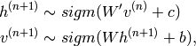
![]() 表示第 n 步 所有隐藏层神经元。比如:
表示第 n 步 所有隐藏层神经元。比如:![]() 根据概率 决定是 0 还是 1;同样地, 根据概率
根据概率 决定是 0 还是 1;同样地, 根据概率![]() 决定是 0 还是 1。
决定是 0 还是 1。
这个过程如下图:

当 ![]() ,样本
,样本![]() 就可以保证是联合概率
就可以保证是联合概率 ![]() 的样本了。说了这么一大堆,目的就是得到满足分布
的样本了。说了这么一大堆,目的就是得到满足分布![]() 的样本,从而估计梯度公式中不好计算的期望项。(博客公式5.45和6.52)
的样本,从而估计梯度公式中不好计算的期望项。(博客公式5.45和6.52)
理论上,训练中每个参数更新都需要进行一次采样,这大大降低了效率。因此,研究人员发明了不少很多算法,在训练过程中,高效地进行对分布 ![]() 进行抽样。
进行抽样。
Contrastive Divergence (CD-k)
这类概括还是原文复制比较好:
Contrastive Divergence uses two tricks to speed up the sampling process:
- since we eventually want (the true, underlying distribution of the data), we initialize the Markov chain with a training example (i.e., from a distribution that is expected to be close(接近) to
 , so that thechain will be already close(接近) to having converged to its final distribution ).
 - CD does not wait for the chain to converge. Samples are obtained after only k-steps of Gibbs sampling. In pratice,
 has been shown to work surprisingly well.
第一点是赋初值,好多迭代的机器学习算法的优化都可以从如何给出良好的初值入手;
第二点是只采样K步,我们不一定非要等到马尔科夫链收敛到最终状态,我们只进行 K 次 吉布斯采样,实践中,K=1 效果都出乎意料地好。
Persistent CD
Persistent CD [Tieleman08] uses another approximation for sampling from ![]() . It relies on a single Markov chain, which has a persistent state (i.e., not restarting a chain for each observed example). For each parameter update, we extract new samples by simply running the chain for k-steps. The state of the chain is then preserved for subsequent updates.
. It relies on a single Markov chain, which has a persistent state (i.e., not restarting a chain for each observed example). For each parameter update, we extract new samples by simply running the chain for k-steps. The state of the chain is then preserved for subsequent updates.
The general intuition is that if parameter updates are small enough compared to the mixing rate of the chain, the Markov chain should be able to “catch up” to changes in the model.
Persistent CD [Tieleman08] 我之前没见过,以后有空再看看论文。
Implementation
我们构造了RBM类。网络参数可以通过构造函数轻松设置。这种模式在构建基于RBM的深度网络时特别有用,和之前自编码器一样,参数权重与MLP的网络层共享(即这里的网络层既可以看成RBM层,也可以看成MLP的网络层,两者的性质都兼具)。
class RBM(object):
    """Restricted Boltzmann Machine (RBM)  """
    def __init__(
        self,
        input=None,
        n_visible=784,
        n_hidden=500,
        W=None,
        hbias=None,
        vbias=None,
        numpy_rng=None,
        theano_rng=None
    ):
        """
        RBM constructor. Defines the parameters of the model along with
        basic operations for inferring hidden from visible (and vice-versa),
        as well as for performing CD updates.

        :param input: None for standalone RBMs or symbolic variable if RBM is
        part of a larger graph.

        :param n_visible: number of visible units

        :param n_hidden: number of hidden units

        :param W: None for standalone RBMs or symbolic variable pointing to a
        shared weight matrix in case RBM is part of a DBN network; in a DBN,
        the weights are shared between RBMs and layers of a MLP

        :param hbias: None for standalone RBMs or symbolic variable pointing
        to a shared hidden units bias vector in case RBM is part of a
        different network

        :param vbias: None for standalone RBMs or a symbolic variable
        pointing to a shared visible units bias
        """

        self.n_visible = n_visible
        self.n_hidden = n_hidden

        if numpy_rng is None:
            # create a number generator
            numpy_rng = numpy.random.RandomState(1234)

        if theano_rng is None:
            theano_rng = RandomStreams(numpy_rng.randint(2 ** 30))

        if W is None:
            # W is initialized with `initial_W` which is uniformely
            # sampled from -4*sqrt(6./(n_visible+n_hidden)) and
            # 4*sqrt(6./(n_hidden+n_visible)) the output of uniform if
            # converted using asarray to dtype theano.config.floatX so
            # that the code is runable on GPU
            initial_W = numpy.asarray(
                numpy_rng.uniform(
                    low=-4 * numpy.sqrt(6. / (n_hidden + n_visible)),
                    high=4 * numpy.sqrt(6. / (n_hidden + n_visible)),
                    size=(n_visible, n_hidden)
                ),
                dtype=theano.config.floatX
            )
            # theano shared variables for weights and biases
            W = theano.shared(value=initial_W, name='W', borrow=True)

        if hbias is None:
            # create shared variable for hidden units bias
            hbias = theano.shared(
                value=numpy.zeros(
                    n_hidden,
                    dtype=theano.config.floatX
                ),
                name='hbias',
                borrow=True
            )

        if vbias is None:
            # create shared variable for visible units bias
            vbias = theano.shared(
                value=numpy.zeros(
                    n_visible,
                    dtype=theano.config.floatX
                ),
                name='vbias',
                borrow=True
            )

        # initialize input layer for standalone RBM or layer0 of DBN
        self.input = input
        if not input:
            self.input = T.matrix('input')

        self.W = W
        self.hbias = hbias
        self.vbias = vbias
        self.theano_rng = theano_rng
        # **** WARNING: It is not a good idea to put things in this list
        # other than shared variables created in this function.
        self.params = [self.W, self.hbias, self.vbias]
根据公式(7):
def propup(self, vis):
        '''This function propagates the visible units activation upwards to
        the hidden units

        Note that we return also the pre-sigmoid activation of the
        layer. As it will turn out later, due to how Theano deals with
        optimizations, this symbolic variable will be needed to write
        down a more stable computational graph (see details in the
        reconstruction cost function)

        '''
        pre_sigmoid_activation = T.dot(vis, self.W) + self.hbias
        return [pre_sigmoid_activation, T.nnet.sigmoid(pre_sigmoid_activation)]
根据上面函数算出的概率,模拟出隐藏层神经元结果:
 def sample_h_given_v(self, v0_sample):
        ''' This function infers state of hidden units given visible units '''
        # compute the activation of the hidden units given a sample of
        # the visibles
        pre_sigmoid_h1, h1_mean = self.propup(v0_sample)
        # get a sample of the hiddens given their activation
        # Note that theano_rng.binomial returns a symbolic sample of dtype
        # int64 by default. If we want to keep our computations in floatX
        # for the GPU we need to specify to return the dtype floatX
        h1_sample = self.theano_rng.binomial(size=h1_mean.shape,
                                             n=1, p=h1_mean,
                                             dtype=theano.config.floatX)
        return [pre_sigmoid_h1, h1_mean, h1_sample]
根据公式(8):
def propdown(self, hid):
        '''This function propagates the hidden units activation downwards to
        the visible units

        Note that we return also the pre_sigmoid_activation of the
        layer. As it will turn out later, due to how Theano deals with
        optimizations, this symbolic variable will be needed to write
        down a more stable computational graph (see details in the
        reconstruction cost function)

        '''
        pre_sigmoid_activation = T.dot(hid, self.W.T) + self.vbias
        return [pre_sigmoid_activation, T.nnet.sigmoid(pre_sigmoid_activation)]
根据上面函数算出的概率,模拟出可见层神经元结果:
def sample_v_given_h(self, h0_sample):
        ''' This function infers state of visible units given hidden units '''
        # compute the activation of the visible given the hidden sample
        pre_sigmoid_v1, v1_mean = self.propdown(h0_sample)
        # get a sample of the visible given their activation
        # Note that theano_rng.binomial returns a symbolic sample of dtype
        # int64 by default. If we want to keep our computations in floatX
        # for the GPU we need to specify to return the dtype floatX
        v1_sample = self.theano_rng.binomial(size=v1_mean.shape,
                                             n=1, p=v1_mean,
                                             dtype=theano.config.floatX)
        return [pre_sigmoid_v1, v1_mean, v1_sample]
定义关于Gibbs sampling(Gibbs 采样)的函数:
gibbs_vhv 函数是从可见层开始,根据公式(7)算出隐藏层,再根据公式(8)算出可见层。 As we shall see, this will be useful for sampling from the RBM.
def gibbs_hvh(self, h0_sample):
        ''' This function implements one step of Gibbs sampling,
            starting from the hidden state'''
        pre_sigmoid_v1, v1_mean, v1_sample = self.sample_v_given_h(h0_sample)
        pre_sigmoid_h1, h1_mean, h1_sample = self.sample_h_given_v(v1_sample)
        return [pre_sigmoid_v1, v1_mean, v1_sample,
                pre_sigmoid_h1, h1_mean, h1_sample]
gibbs_hvh 函数是从隐藏层开始,根据公式(8)算出可见层,再根据公式(7)算出隐藏层。 This function will be useful for performing CD and PCD updates.
 def gibbs_vhv(self, v0_sample):
        ''' This function implements one step of Gibbs sampling,
            starting from the visible state'''
        pre_sigmoid_h1, h1_mean, h1_sample = self.sample_h_given_v(v0_sample)
        pre_sigmoid_v1, v1_mean, v1_sample = self.sample_v_given_h(h1_sample)
        return [pre_sigmoid_h1, h1_mean, h1_sample,
                pre_sigmoid_v1, v1_mean, v1_sample]

    # start-snippet-2
这段说明了为什么让函数返回 pre-sigmoid activation:(目的是为了Theano能识别到,然后优化计算)
Note that we also return the pre-sigmoid activation(sigmoid函数括号里的值).To understand why this is so you need to understand a bit about how Theano works. Whenever you compile a Theano function, the computational graph that you pass as input gets optimized for speed and stability. This is done by changing several parts of the subgraphs with others. One such optimization expresses terms of the form log(sigmoid(x)) in terms of softplus. We need this optimization for the cross-entropy since sigmoid of numbers larger than 30. (or even less then that) turn to 1. and numbers smaller than -30. turn to 0 which in terms will force theano to compute log(0) and therefore we will get either -inf or NaN as cost. If the value is expressed in terms of softplus we do not get this undesirable behaviour.
This optimization usually works fine, but here we have a special case. The sigmoid is applied inside the scan op, while the log is outside. Therefore Theano will only see log(scan(..)) instead of log(sigmoid(..))and will not apply the wanted optimization. We can not go and replace the sigmoid in scan with something else also,because this only needs to be done on the last step. Therefore the easiest and more efficient way is to get also the pre-sigmoid activation as an output of scan, and apply both the log and sigmoid outside scan such that Theano can catch and optimize the expression.
计算参数梯度时需要计算 the free energy of the model,公式(9),注意是在![]() and
and![]() 情况下推出的公式,代码如下,返回 pre-sigmoid:
情况下推出的公式,代码如下,返回 pre-sigmoid:
def free_energy(self, v_sample):
        ''' Function to compute the free energy '''
        wx_b = T.dot(v_sample, self.W) + self.hbias
        vbias_term = T.dot(v_sample, self.vbias)
        hidden_term = T.sum(T.log(1 + T.exp(wx_b)), axis=1)
        return -hidden_term - vbias_term
构建一个 get_cost_updates 函数, 来生成 CD-k and PCD-k 算法更新参数所需的梯度:
def get_cost_updates(self, lr=0.1, persistent=None, k=1):
        """This functions implements one step of CD-k or PCD-k

        :param lr: learning rate used to train the RBM

        :param persistent: None for CD. For PCD, shared variable
            containing old state of Gibbs chain. This must be a shared
            variable of size (batch size, number of hidden units).

        :param k: number of Gibbs steps to do in CD-k/PCD-k

        Returns a proxy for the cost and the updates dictionary. The
        dictionary contains the update rules for weights and biases but
        also an update of the shared variable used to store the persistent
        chain, if one is used.

        """

        # compute positive phase
        pre_sigmoid_ph, ph_mean, ph_sample = self.sample_h_given_v(self.input)

        # decide how to initialize persistent chain:
        # for CD, we use the newly generate hidden sample
        # for PCD, we initialize from the old state of the chain
        if persistent is None:
            chain_start = ph_sample
        else:
            chain_start = persistent
注意 此函数有一个参数 persistent 。这是为了让代码适用于 CD 和 PCD 两种算法。
当使用PCD时,persistent 被设置为共享变量,值为上一次迭代Gibbs chain的状态(PCD详见Persistent CD[Tieleman08])。
当 persistent 为 None 时,我们用函数 sample_h_given_v 初始化隐藏层神经元,然后运行 CD 算法。一旦我们初始化了 Gibbs chain ,就可以一直迭代计算到收敛,为公式(4)采样。To do so, we will use thescan op provided by Theano, therefore we urge the reader to look it up by following thislink.
# perform actual negative phase
        # in order to implement CD-k/PCD-k we need to scan over the
        # function that implements one gibbs step k times.
        # Read Theano tutorial on scan for more information :
        # http://deeplearning.net/software/theano/library/scan.html
        # the scan will return the entire Gibbs chain
        (
            [
                pre_sigmoid_nvs,
                nv_means,
                nv_samples,
                pre_sigmoid_nhs,
                nh_means,
                nh_samples
            ],
            updates
        ) = theano.scan(
            self.gibbs_hvh,
            # the None are place holders, saying that
            # chain_start is the initial state corresponding to the
            # 6th output
            outputs_info=[None, None, None, None, None, chain_start],
            n_steps=k
        )
一旦我们生成了 Gibbs chain 且在链尾采样来得到 free energy of the negative phase (见公式(4))。注意:thechain_end is a symbolical Theano variable expressed in terms of the model parameters, 如果我们直接使用T.grad ,the function will try to go through the Gibbs chain to get the gradients. This is not what we want (it will mess up our gradients) and therefore we need to indicate to T.grad that chain_end is a constant. We do this by using the argumentconsider_constant ofT.grad.
# determine gradients on RBM parameters
        # note that we only need the sample at the end of the chain [-1]表示取最后一个
        chain_end = nv_samples[-1]

        cost = T.mean(self.free_energy(self.input)) - T.mean(
            self.free_energy(chain_end))
        # We must not compute the gradient through the gibbs sampling
        gparams = T.grad(cost, self.params, consider_constant=[chain_end])
教程前面提到了关于 cost(损失函数)用的 negative log-likelihood,这里代码就是按照此公式来的(或者看 不对参数求导的公式(4)):
最后,我们得到了存有权重如何更新的字典 updates ,这个updates 是由 scan 返回的。如果使用 PCD 算法,这个字典里还保存了 the state of the Gibbs chain(因为PCD需要接着链的状态继续运行)。
# constructs the update dictionary
        for gparam, param in zip(gparams, self.params):
            # make sure that the learning rate is of the right dtype
            updates[param] = param - gparam * T.cast(
                lr,
                dtype=theano.config.floatX
            )
        if persistent:
            # Note that this works only if persistent is a shared variable
            updates[persistent] = nh_samples[-1]
            # pseudo-likelihood is a better proxy for PCD
            monitoring_cost = self.get_pseudo_likelihood_cost(updates)
        else:
            # reconstruction cross-entropy is a better proxy for CD
            monitoring_cost = self.get_reconstruction_cost(updates,
                                                           pre_sigmoid_nvs[-1])

        return monitoring_cost, updates
注意 monitoring_cost