机器学习--线性回归、逻辑回归

一、线性回归

线性回归无非就是训练得到线性函数的参数来回归出一个线性模型，学习《最优化方法》时中的最小二乘问题就是线性回归的问题。

关于线性回归，ng老师的视频里有讲，也可以看此博客单参数线性回归。简要说一下线性回归的原理。

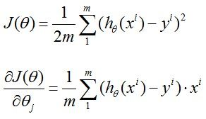
假设拟合直线为h(x)=θ0+θ1*x, 记Cost Function为J(θ0,θ1)

这其实就是一个线性回归问题，上式也是一个最小二乘问题的模型。盗的图，我认为式中1/m完全没必要，还增加运算，完全可以删掉。线性回归就是要用数据训练出来参数θ，训练时要使目标函数最小，其中x(i)和y(i)中的i表示第i条样本数据，这就是一个无约束优化的问题，关于无约束优化问题的解决方法有很多，比如梯度下降，共轭梯度、牛顿法、步长加速法等等。关于无约束优化和最小二乘问题可以看《最优化方法》相关的书，都有很详细的讲解。这里用最简单的梯度下降。

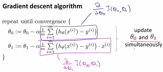
需要朝着目标函数J梯度下降的方向迭代更行参数θ，

由此

以上就是线性回归了。

二、逻辑回归

线性回归能到一个模型来进行预测，要想用来分类，就要用到逻辑回归。

要分类，就要把h(x)的结果限制在0~1范围内,引入sigmoid函数

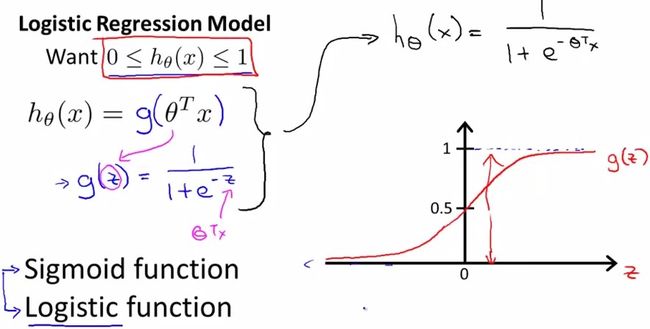
假设我们的样本是{x, y}，y是0或者1，表示正类或者负类，x是我们的m维的样本特征向量。那么这个样本x属于正类，也就是y=1的“概率”可以通过下面的逻辑函数来表示：

所以说，LogisticRegression 就是一个被logistic方程归一化后的线性回归，仅此而已。

怎么来构造代价函数，就用到最大似然，关于最大似然估计，本科概率论有相关知识。

假设我们有n个独立的训练样本{(x₁, y₁) ,(x₂, y₂),…, (x_n, y_n)}，y={0, 1}。那每一个观察到的样本(x_i, y_i)出现的概率是：

那最大似然法就是求模型中使得似然函数最大的系数取值θ*。这个最大似然就是我们的代价函数（cost function）了。

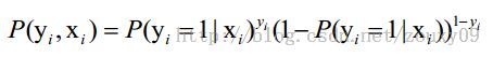
这时候，用L(θ)对θ求导，得到：

下一步要做的就是优化求解了。所以以上都只是推导过程， 真正用到的就是这个式子 。

三、优化

这一块可以看这篇博客逻辑回归，讲的很细。其实该篇博客主要内容来自《机器学习实战》

注意梯度下降和随机梯度下降的区别。梯度下降每一次迭代都要把整个数据来求导，随即梯度下降则是每一次迭代只用一个样本数据，梯度下降适合小数据，随即梯度下降适合大数据集。

四、总结

所以其实逻辑回归实现时真正用到的就是

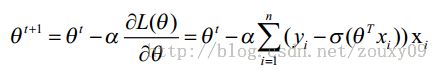
每一次对上式迭代

关于matlab代码，上面博客作者的博客里有相关代码，但她是调用了无约束优化的相关函数，所以实现很简单，另外关于正则化的实现我认为她代码不对

上面的博客里有python的代码，《机器学习实战》也有。

#################################################
# logRegression: Logistic Regression
# Author : zouxy
# Date   : 2014-03-02
# HomePage : http://blog.csdn.net/zouxy09
# Email  : [email protected]
#################################################

from numpy import *
import matplotlib.pyplot as plt
import time


# calculate the sigmoid function
def sigmoid(inX):
    return 1.0 / (1 + exp(-inX))


# train a logistic regression model using some optional optimize algorithm
# input: train_x is a mat datatype, each row stands for one sample
#        train_y is mat datatype too, each row is the corresponding label
#        opts is optimize option include step and maximum number of iterations
def trainLogRegres(train_x, train_y, opts):
    # calculate training time
    startTime = time.time()

    numSamples, numFeatures = shape(train_x)
    alpha = opts['alpha']; maxIter = opts['maxIter']
    weights = ones((numFeatures, 1))

    # optimize through gradient descent algorilthm
    for k in range(maxIter):
        if opts['optimizeType'] == 'gradDescent': # gradient descent algorilthm
            output = sigmoid(train_x * weights)
            error = train_y - output
            weights = weights + alpha * train_x.transpose() * error
        elif opts['optimizeType'] == 'stocGradDescent': # stochastic gradient descent#对于大数据集就不要让随即梯度下降在k循环下循环了，
            for i in range(numSamples):
                output = sigmoid(train_x[i, :] * weights)
                error = train_y[i, 0] - output
                weights = weights + alpha * train_x[i, :].transpose() * error
        elif opts['optimizeType'] == 'smoothStocGradDescent': # smooth stochastic gradient descent
            # randomly select samples to optimize for reducing cycle fluctuations
            dataIndex = range(numSamples)
            for i in range(numSamples):
                alpha = 4.0 / (1.0 + k + i) + 0.01
                randIndex = int(random.uniform(0, len(dataIndex)))
                output = sigmoid(train_x[randIndex, :] * weights)
                error = train_y[randIndex, 0] - output
                weights = weights + alpha * train_x[randIndex, :].transpose() * error
                del(dataIndex[randIndex]) # during one interation, delete the optimized sample
        else:
            raise NameError('Not support optimize method type!')


    print 'Congratulations, training complete! Took %fs!' % (time.time() - startTime)
    return weights


# test your trained Logistic Regression model given test set
def testLogRegres(weights, test_x, test_y):
    numSamples, numFeatures = shape(test_x)
    matchCount = 0
    for i in xrange(numSamples):
        predict = sigmoid(test_x[i, :] * weights)[0, 0] > 0.5
        if predict == bool(test_y[i, 0]):
            matchCount += 1
    accuracy = float(matchCount) / numSamples
    return accuracy


# show your trained logistic regression model only available with 2-D data
def showLogRegres(weights, train_x, train_y):
    # notice: train_x and train_y is mat datatype
    numSamples, numFeatures = shape(train_x)
    if numFeatures != 3:
        print "Sorry! I can not draw because the dimension of your data is not 2!"
        return 1

    # draw all samples
    for i in xrange(numSamples):
        if int(train_y[i, 0]) == 0:
            plt.plot(train_x[i, 1], train_x[i, 2], 'or')
        elif int(train_y[i, 0]) == 1:
            plt.plot(train_x[i, 1], train_x[i, 2], 'ob')

    # draw the classify line
    min_x = min(train_x[:, 1])[0, 0]
    max_x = max(train_x[:, 1])[0, 0]
    weights = weights.getA()  # convert mat to array
    y_min_x = float(-weights[0] - weights[1] * min_x) / weights[2]
    y_max_x = float(-weights[0] - weights[1] * max_x) / weights[2]
    plt.plot([min_x, max_x], [y_min_x, y_max_x], '-g')
    plt.xlabel('X1'); plt.ylabel('X2')
    plt.show()

#################################################
# logRegression: Logistic Regression
# Author : zouxy
# Date   : 2014-03-02
# HomePage : http://blog.csdn.net/zouxy09
# Email  : [email protected]
#################################################

from numpy import *
import matplotlib.pyplot as plt
import time
from logregression import trainLogRegres,testLogRegres,showLogRegres
def loadData():
    train_x = []
    train_y = []
    fileIn = open('E:/Python/Machine Learning in Action/testSet.txt')
    for line in fileIn.readlines():
        lineArr = line.strip().split()
        train_x.append([1.0, float(lineArr[0]), float(lineArr[1])])#追加内容
        train_y.append(float(lineArr[2]))
    return mat(train_x), mat(train_y).transpose()


## step 1: load data
print "step 1: load data..."
train_x, train_y = loadData()
test_x = train_x; test_y = train_y

## step 2: training...
print "step 2: training..."
opts = {'alpha': 0.01, 'maxIter': 20, 'optimizeType': 'smoothStocGradDescent'}#字典
optimalWeights = trainLogRegres(train_x, train_y, opts)

## step 3: testing
print "step 3: testing..."#新版本要加括号
accuracy = testLogRegres(optimalWeights, test_x, test_y)

## step 4: show the result
print "step 4: show the result..."
print 'The classify accuracy is: %.3f%%' % (accuracy * 100)
showLogRegres(optimalWeights, train_x, train_y)

数据集

-0.017612   14.053064   0
-1.395634   4.662541    1
-0.752157   6.538620    0
-1.322371   7.152853    0
0.423363    11.054677   0
0.406704    7.067335    1
0.667394    12.741452   0
-2.460150   6.866805    1
0.569411    9.548755    0
-0.026632   10.427743   0
0.850433    6.920334    1
1.347183    13.175500   0
1.176813    3.167020    1
-1.781871   9.097953    0
-0.566606   5.749003    1
0.931635    1.589505    1
-0.024205   6.151823    1
-0.036453   2.690988    1
-0.196949   0.444165    1
1.014459    5.754399    1
1.985298    3.230619    1
-1.693453   -0.557540   1
-0.576525   11.778922   0
-0.346811   -1.678730   1
-2.124484   2.672471    1
1.217916    9.597015    0
-0.733928   9.098687    0
-3.642001   -1.618087   1
0.315985    3.523953    1
1.416614    9.619232    0
-0.386323   3.989286    1
0.556921    8.294984    1
1.224863    11.587360   0
-1.347803   -2.406051   1
1.196604    4.951851    1
0.275221    9.543647    0
0.470575    9.332488    0
-1.889567   9.542662    0
-1.527893   12.150579   0
-1.185247   11.309318   0
-0.445678   3.297303    1
1.042222    6.105155    1
-0.618787   10.320986   0
1.152083    0.548467    1
0.828534    2.676045    1
-1.237728   10.549033   0
-0.683565   -2.166125   1
0.229456    5.921938    1
-0.959885   11.555336   0
0.492911    10.993324   0
0.184992    8.721488    0
-0.355715   10.325976   0
-0.397822   8.058397    0
0.824839    13.730343   0
1.507278    5.027866    1
0.099671    6.835839    1
-0.344008   10.717485   0
1.785928    7.718645    1
-0.918801   11.560217   0
-0.364009   4.747300    1
-0.841722   4.119083    1
0.490426    1.960539    1
-0.007194   9.075792    0
0.356107    12.447863   0
0.342578    12.281162   0
-0.810823   -1.466018   1
2.530777    6.476801    1
1.296683    11.607559   0
0.475487    12.040035   0
-0.783277   11.009725   0
0.074798    11.023650   0
-1.337472   0.468339    1
-0.102781   13.763651   0
-0.147324   2.874846    1
0.518389    9.887035    0
1.015399    7.571882    0
-1.658086   -0.027255   1
1.319944    2.171228    1
2.056216    5.019981    1
-0.851633   4.375691    1
-1.510047   6.061992    0
-1.076637   -3.181888   1
1.821096    10.283990   0
3.010150    8.401766    1
-1.099458   1.688274    1
-0.834872   -1.733869   1
-0.846637   3.849075    1
1.400102    12.628781   0
1.752842    5.468166    1
0.078557    0.059736    1
0.089392    -0.715300   1
1.825662    12.693808   0
0.197445    9.744638    0
0.126117    0.922311    1
-0.679797   1.220530    1
0.677983    2.556666    1
0.761349    10.693862   0
-2.168791   0.143632    1
1.388610    9.341997    0
0.317029    14.739025   0

五、在分布式系统中实现

关于lr在maprudece中的实现，logistic regression不支持并行，也就是mahout实现的也是单机的，运行在hadoop上面也没有意义（个人观点）。

看mahout中的源码分析：mahout源码分析之logistic regression（2）--RunLogistic

参考文献：

[1].  Ng机器学习视频

[2]. 机器学习实战

[3]. Stanford机器学习---第三讲. 逻辑回归和过拟合问题的解决 logistic Regression & Regularization

[4]. 机器学习算法与Python实践之（七）逻辑回归（Logistic Regression）