机器学习之AdaBoost元算法（七）

主要内容：
● 组合相似的分类器来提高分类器性能
● 应用AdaBoost算法
● 处理非均衡问题分类问题

打个比方， 做重要决定的时候， 大家可能会汲取多个专家而不是一个人的意见。机器学习处理处理问题的时候，也是如此，这就是元算法的思路。
元算法是对其他算法进行组合的一种方式。

7.1 基于数据集多重抽样的分类器
前面介绍了五种不同的算法，各有优缺点。我们可以将不同的分类器组合起来，这种组合结果被称之为集成方法或者元算法。 使用集成方法可以有很多形式，可以是不同算法的集成，也可以是同一算法在不同的设置下的集成， 还可以是数据集不同部分分配给不同分类器之后的集成。

AdaBoost
优点：泛化错误率低，可以应用到大部分分类器上，无参数调整。
缺点：对离群点敏感
适用数据类型：数值型和标称型数据。

7.1.1 bagging：基于数据随机抽样的分类器的构建方法

自举汇聚法，或称bagging方法 。 是在原始数据集中选择S次后得到S个新数据集的一种技术。新数据集和原始数据集的大小相等。

7.1.2 boosting
boosting是通过集中关注被已有的分类器错分的那些数据来获得新的分类器。
boosting有多个版本，我们现在只讨论AdaBoost。

AdaBoost的一般流程：
（1）收集数据：可以使用任意方法
（2）准备数据：依赖于所使用的弱分类器类型，本次使用的是单层决策树，这种分类器可以处理任何数据类型。还可以使用任意分类器作为弱分类器。其中，kNN，决策树，朴素贝叶斯，logistic回归，支持向量机任一分类器都可以充当分类器。作为弱分类器，简单分类器的效果会更好。
（3）分析数据：可以使用任意方法
（4）训练算法：AdaBoost的大部分时间都在训练上，分类器将多次在同一数据集上训练弱分类器。
（5）测试算法：计算分类的错误率
（6）使用算法：同SVM一样，AdaBoost预测两个类别中的一个。如果想把它应用到多个类别的场合，那么就要像多类SVM中的做法一样，对AdaBoost代码进行修改。

7.2 训练算法：基于错误提升分类器的性能
能不能用弱分类器和多个实例来构建一个强分类器。
在二分类的情况下弱分类的错误率会高于50% ，而强分类器的错误率会低很多。

AdaBoost（adaptive boosting ：自适应）的缩写。运行过程如下：
1. 训练数据中的每个样本，赋予一个权重，这些权重构成了向量D。
2. 一开始，这些权重都初始化成相等值，首先在训练数据上训练出一个弱分类器的并计算该分类器的错误率，然后在同一数据集上再次训练弱分类器。
3.在分类器第二次训练当中，将会重新调整每个样本的权重，其中第一次分对的样本的权重会降低，而第一次分错的样本的权重将会提高。
4.为了从所有弱分类器中得到最终的分类结果，AdaBoost为每个分类器都配了一个权重值alpha，这些alpha值是基于每个弱分类器的错误率进行计算的。
其中，错误率 ε 定义为：

ε = 未正确分类的样本数目 / 所有的样本数目

其中，alpha的公式如下

a = ln(1-ε\ε) * 1\2

AdaBoost算法的流程图如下：

计算出alpha 之后，可以对权重向量D进行更新，使得正确分类的样本权重降低而错分样本的权重升高。
如果某个样本被正确分类，那么该样本的权重更改为：

计算出D之后，AdaBoost算法会进行下一次迭代。算法不断重复训练和调整权重的过程，直到训练错误率为0或者弱分类的数目达到用户的指定值为止。

7.3 基于单层决策树构建弱分类器

单层决策树（decision stump，也称之为决策树桩）是一种简单的决策树。这个单层决策树仅基于单个特征的来做决策。

我们将使用多套代码来构建单层决策树：
1.第一个函数将用于测试是否有某个值小于或者大于我们正在测试的阈值。
2.第二个函数在一个加权平均数据集中循环，并找到具有最低错误率的单层决策树。

import numpy as np

def loadSimpData():
    datMat = np.matrix(
            [[ 1. , 2.1],
             [ 2. , 1.1],
             [ 1.3, 1. ],
             [ 1. , 1. ],
             [ 2. , 1. ]])
    classLabels = [1.0 , 1.0, -1.0, -1.0, 1.0]
    return datMat, classLabels

第二个函数的伪代码如下：

""" 将最小错误率minError设为 +inf 大 对数据集中的每一个特征(第一层循环)： 对每个步长(第二层循环)： 对每个不等号(第三层循环)： 建立一棵单层决策树并利用加权数据集对它进行测试 如果错误率地域minError，则将当前的单层决策树设为最佳单位决策树 返回最佳单层决策树 """

#=========================================================================
# 单层决策树生成函数
def stumpClassify(dataMatrix, dimen, threshVal, threshIneq):
    retArray = np.ones((np.shape(dataMatrix)[0],1))
    if threshIneq == 'lt':
        retArray[dataMatrix[:, dimen] <= threshVal] = -1.0
    else:
        retArray[dataMatrix[:, dimen] > threshVal] = 1.0
    return retArray

def buildStump(dataArr, classLabels, D):
    dataMatrix = np.mat(dataArr); labelMat = np.mat(classLabels).T
    m, n = np.shape(dataMatrix)                    
    numSteps = 10.0; bestStump = {}; bestClasEst = np.mat(np.zeros((m, 1)))
    minError = inf
    for i in range(n):
        rangeMin = dataMatrix[:, i].min();rangeMax = dataMatrix[:, 1].max()
        stepSize = (rangeMax - rangeMin)/numSteps
        for j in range(-1, int(numSteps) + 1):
            for inequal in ['lt', 'gt']:
                threshVal = (rangeMin + float(j) * stepSize)
                predictedVals = stumpClassify(dataMatrix, i, threshVal, inequal)
                errArr = np.mat(np.ones((m, 1)))
                errArr[predictedVals == labelMat] = 0
                weightedError = D.T * errArr
                print "split: dim %d, thresh %.2f, thresh inequal: %s, the weighted error is %.3f" %(i ,threshVal, inequal,weightedError)
                if weightedError < minError:
                    minError = weightedError
                    bestClasEst = predictedVals.copy()
                    bestStump['dim'] = i
                    bestStump['thresh'] = threshVal
                    bestStump['ineq'] = inequal
    return bestStump, minError, bestClasEst

至此，我们构架了一个基于加权输入值进行决策的分类器。

1。第一个函数stumpClassify()是通过阈值比较对数据进行分类的。所有在阈值一边的数据会分到类别-1，而在另一边的数据会分到类别+1 ，。该函数可以通过数组过滤来实现，，将返回的数组的全部元素设置为+1，然后将所有不满足不等式要求的元素设置为-1 。
2.第二个函数buildStump() 将遍历buildStump()函数所有可能输入的值，并找到数据集上最佳的单层决策树。（“最佳”是基于权重向量D来定义的），bestStump这个空字典集用于存储给定权重向量D所得到的最佳单层决策树的相关信息。minError 正无穷大，用于寻找可能的最小概率。
3.三层嵌套的for循环是程序的最主要的部分。第一层for循环在数据集的所有特征上遍历。通过计算最小值和最大值来了解需要最大的步长。第二层for循环在这些特征的值上进行遍历。最后一个for循环是在大于和小于之间切换不等式。
4.在三层的for循环之内，我们在数据集及三个循环变量上调用stumpClassify()函数。构建的列向量errArr，若predictedVals中的值不等于labelMat中的真正类别的标签值，errArr = 1。
errArr 和权重向量D乘积相应元素求和，得到weightedError。
5.我们是基于权重向量D而不是其他错误计算指标来评价分类器的。

In [7]: import adaboost

In [8]: reload(adaboost)
Out[8]: <module 'adaboost' from 'adaboost.py'>

In [9]: datMat, classLabels = adaboost.loadSimpData()
    ...:
In [15]: D = np.mat(np.ones((5,1))/5)

In [16]: D
Out[16]:
matrix([[ 0.2], [ 0.2], [ 0.2], [ 0.2], [ 0.2]])

In [17]: adaboost.buildStump(datMat,classLabels,D)
split: dim 0, thresh 0.89, thresh inequal: lt, the weighted error is 0.400
split: dim 0, thresh 0.89, thresh inequal: gt, the weighted error is 0.400
split: dim 0, thresh 1.00, thresh inequal: lt, the weighted error is 0.400
split: dim 0, thresh 1.00, thresh inequal: gt, the weighted error is 0.400
......
split: dim 1, thresh 1.88, thresh inequal: gt, the weighted error is 0.400
split: dim 1, thresh 1.99, thresh inequal: lt, the weighted error is 0.400
split: dim 1, thresh 1.99, thresh inequal: gt, the weighted error is 0.400
split: dim 1, thresh 2.10, thresh inequal: lt, the weighted error is 0.600
split: dim 1, thresh 2.10, thresh inequal: gt, the weighted error is 0.400
Out[17]:
({'dim': 0, 'ineq': 'lt', 'thresh': 1.3300000000000001},
matrix([[ 0.2]]),
array([[-1.], [ 1.], [-1.], [-1.], [ 1.]]))

上述的单层决策树的生成函数是决策树的一个简化版本。也就是弱分类算法。

7.4 完整的AdaBoos 算法实现
我们将利用构建的单层决策树来实现这个完整算法。

伪代码：

""" 对每次迭代： 利用buildStump()函数找到最佳的单层决策树 将最佳单层决策树加入到单层决策树数组 计算alpha 计算新的权重向量D 更新累计类别估计值 如果错误率为0.0 ， 则退出循环 """

#基于单层决策树的AdaBoost训练过程
def adaboostTrainDS(dataArr, classLabels, numIt = 40):
    """ 数据集，类别标签，迭代次数 """
    weakClassArr = []
    m = np.shape(dataArr)[0]
    D = np.mat(np.ones((m, 1))/m)
    aggClassEst = np.mat(np.zeros((m, 1)))
    for i in range(numIt):
        bestStump, error, classEst = buildStump(dataArr, classLabels, D)
        print "D:", D.T
        alpha = float(0.5*np.log((1.0-error)/max(error, 1e-16)))
        bestStump['alphas'] = alpha
        weakClassArr.append(bestStump)
        print "classEst:",classEst.T
        expon = np.multiply(-1*alpha*np.mat(classLabels).T, classEst)
        D = np.multiply(D,np.exp(expon))
        D = D/D.sum()
        aggClassEst += alpha*classEst
        print "aggClassEst: ",aggClassEst.T
        aggErrors = np.multiply(np.sign(aggClassEst) != np.mat(classLabels).T, np.ones((m, 1)))
        ErrorRate = aggErrors.sum()/m
        print "total error:",ErrorRate,"\n"
        if ErrorRate ==0.0:
            break
    return weakClassArr

1.函数名称尾部的DS代表的就是单层决策树，是adaboost中最流行的弱分类器。
2.向量D非常重要，包含了每个数据点的权重。这些权重都赋予了相等的值，后续的迭代中，adaboost算法会增加错分数据的权重同时，降低正确分类的数据的权重。
3.adaboost 算法的核心在于for循环，该循环运行numTt次或者直到训练错误率为0为止。
4.alpha值会告诉分类器本次单层决策树输出结果的权重。其中max(error, 1e-16)用于确保没有错误的时候不会发生除零溢出。

In [52]: import adaboost

In [53]: reload(adaboost)
Out[53]: <module 'adaboost' from 'adaboost.pyc'>
In [55]: classifierArray = adaboost.adaboostTrainDS(datMat,classLabels,9)
split: dim 0, thresh 0.89, thresh inequal: lt, the weighted error is 0.400
split: dim 0, thresh 0.89, thresh inequal: gt, the weighted error is 0.400
......
split: dim 1, thresh 2.10, thresh inequal: lt, the weighted error is 0.600
split: dim 1, thresh 2.10, thresh inequal: gt, the weighted error is 0.400
D: [[ 0.2 0.2 0.2 0.2 0.2]]
classEst: [[-1. 1. -1. -1. 1.]]
aggClassEst: [[-0.69314718 0.69314718 -0.69314718 -0.69314718 0.69314718]]
total error: 0.2
......
split: dim 0, thresh 0.89, thresh inequal: gt, the weighted error is 0.143
split: dim 0, thresh 1.00, thresh inequal: lt, the weighted error is 0.357
......
split: dim 1, thresh 2.10, thresh inequal: lt, the weighted error is 0.857
split: dim 1, thresh 2.10, thresh inequal: gt, the weighted error is 0.143
D: [[ 0.28571429 0.07142857 0.07142857 0.07142857 0.5 ]]
classEst: [[ 1. 1. 1. 1. 1.]]
aggClassEst: [[ 1.17568763 2.56198199 -0.77022252 -0.77022252 0.61607184]]
total error: 0.0

观察classifierArray 的值,字典中包含了分类需要的所有信息。

In [58]: classifierArray Out[58]: [{'alphas': 0.6931471805599453, 'dim': 0, 'ineq': 'lt', 'thresh': 1.3300000000000001}, {'alphas': 0.9729550745276565, 'dim': 1, 'ineq': 'lt', 'thresh': 1.0}, {'alphas': 0.8958797346140273, 'dim': 0, 'ineq': 'lt', 'thresh': 0.89000000000000001}]

7.5 测试算法：基于AdaBoost 的分类
每个弱分类器的结果以其对应的alpha值作为权重，所有的弱分类器的结果加权求和就得到了最后的结果。

# AdaBoost分类函数
def adaClassify(datToClass, classifierArr):
    dataMatrix =np.mat(datToClass)
    m = np.shape(dataMatrix)[0]
    aggClassEst = np.mat(np.zeros((m, 1)))
    for i in range(len(classifierArr)):
        classEst = stumpClassify(dataMatrix,classifierArr[i]['dim'],classifierArr[i]['thresh'],classifierArr[i]['ineq'])
        aggClassEst += classifierArr[i]['alphas']*classEst
        print aggClassEst
    return np.sign(aggClassEst) 

adaClassify()函数就是利用训练出的多个弱分类器进行分类的函数。

In [4]: import adaboost

In [5]: reload(adaboost)
Out[5]: <module 'adaboost' from 'adaboost.pyc'>

In [6]: dataArr, labelArr = adaboost.loadSimpData()

In [7]: classifierArr = adaboost.adaboostTrainDS(dataArr,labelArr,30)

In [13]: adaboost.adaClassify([0,0],classifierArr)
[[-0.69314718]]
[[-1.66610226]]
[[-2.56198199]]
Out[13]: matrix([[-1.]])

随着迭代的进行，数据点[0,0]的分类结果越来越强。

In [14: adaboost.adaClassify(([5,5],[0,0]),classifierArr)
[[ 0.69314718] [-0.69314718]]
[[ 1.66610226] [-1.66610226]]
[[ 2.56198199] [-2.56198199]]
Out[14]:
matrix([[ 1.], [-1.]])

这两个点的分类结果也会随着迭代的进行而越来越强。

7.6 示例：在一个难数据集上应用AdaBoost

我们现在想利用多个单层决策树和AdaBoost来预测马疝病死亡率。

示例：在一个难数据集上的AdaBoost应用
1.收集数据：提供的文本文件
2.准备数据：确保类别标签是+1和-1 而不是0和1
3.分析数据：手工检查数据
4.训练算法：在数据上，利用adaBoostTrain() 函数训练出一系列的分类器
5.测试算法：我们拥有两个数据集。在不采用随机抽样的方法下，我们就会对AdaBoost和Logistic回归的结果进行完全对等的比较。
6.使用算法：观察该例子上的错误率。不过，也可构建一个Web网站，让驯马师输入马的病症然后预测马是否会死去。

我们给出一个向文件中加载数据的方法。

# 自适应数据加载函数
def loadDataSet(fileName):
""" 函数能够自检出特征的数目 """
    numFeat = len(open(fileName).readline().split('\t'))
    dataMat = []; labelMat = []
    fr = open(fileName)
    for line in fr.readlines():
        lineArr = []
        curLine = line.strip().split('\t')
        for i in range(numFeat - 1):
            lineArr.append(float(curLine[i]))
        dataMat.append(lineArr)
        labelMat.append(float(curLine[-1]))
    return dataMat, labelMat

上述函数能够自检出特征的数目，函数还能假定最后一个特征是类别标签。

In [26]: dataArr, labelArr = adaboost.loadDataSet(r"E:\ML\ML_source_code\mlia\Ch05\horseColicTraining.txt")

In [29]: classifierArray = adaboost.adaboostTrainDS(dataArr, labelArr,10)
error is 0.986
split: dim 20, thresh 6.30, thresh inequal: gt, the weighted error is 0.500
split: dim 20, thresh 7.20, thresh inequal: lt, the weighted error is 0.997
......
split: dim 20, thresh 9.00, thresh inequal: lt, the weighted error is 1.000
split: dim 20, thresh 9.00, thresh inequal: gt, the weighted error is 0.500
D: [[ 0.00413067 0.00413067 0.00281005 ..., 0.00413067 0.00281005 0.00413067]]
classEst: [[ 1. 1. 1. ..., 1. 1. 1.]]
aggClassEst: [[ 0.38561606 0.38561606 0.38561606 ..., 0.38561606 0.38561606 0.38561606]]
total error: 0.404682274247

In [29]: testArr, testlabelArr = adaboost.loadDataSet(r"E:\ML\ML_source_code\mlia\Ch05\horseColicTest.txt")

In [44]: prediction10 = adaboost.adaClassify(testArr,classifierArray)
[[ 0.1929965] [ 0.1929965] [ 0.1929965] ..., [ 0.38561606] [ 0.38561606] [ 0.38561606]]

In [45]: errArr = np.mat(np.ones((67,1)))

In [46]: errArr[prediction10 != np.mat(testlabelArr).T].sum()
Out[46]: 20.0

将弱分类器的数目设定为1到10000之间的几个不同的数字，运行上述过程。

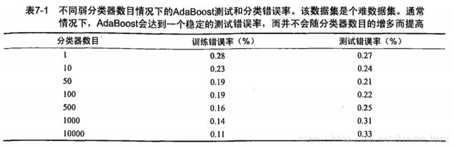
观察上表，我们发现错率达到一个最小值后又开始上升，这称之为 过拟合(overfitting，也称过学习)，

7.7 非均衡分类问题

在前几张的分类器构造里面，我们最终讨论的都是错误率。如果有人牵过来一匹马，让我们预测他是否会生存，我们说马会死，可能马很可能被实施安乐死。我们的预测也许是错误的，马也许本来可以继续活着。但是坦白的说，大多数情况下不同类别的分类代价并不相等。

7.7.1 其他分类器性能度量指标：正确率、召回率、以及ROC曲线

在之前的讨论中，我们都是基于错误率来衡量分类器任务的成功程度的。错误率指的是在所有的测试样本样例中错分的样本的比例。实际上这样的度量错误的掩饰了样例如何被分错误的事实。
在机器学习中的，有一个普遍称之为混淆矩阵的工具，可以帮助人们更好的了解分类中的错误，

在下面这个二类问题中，如果将一个正例判别为正例，那么就认为产生了一个真正例(True , Positive ，TP , 也称之为真阳)；若对一个反例正确的判为反例，就认为产生了一个真反例(True ， Negitive，也称之为真阴)，另外两只情况分别称伪反例(FN ， 假阴)和伪正例(FP ，假阳)。

在分类中，当某个指标的重要性高于其他类别时候，我们就可以利用上述定义来定义出多个比错误率更好的新指标。
第一个指标是正确率（precision），它等于 TP/( TP + FP ) ，给出的是预测能力为正例的样本中的真正正例的比例。
第二个是召回率 （Recall），它等于 TP/( TP + FN ) ， 给出的是预测能力为正例的真实比例占所有真实比例的比例。
在召回率很大的f分类器中，真正判错正例的数目并不多。
另一个用于度量分类中的非均衡性的工具是ROC曲线(ROC curce)，ROC代表接收者操作特征（receiver operating characterristic）。

上图的RCO曲线中，给出了一条虚线和一条实线。虚线给出的是随机猜测的结果曲线。
横坐标轴是伪正例的比例（假阳率=FP/(FP + TN)），而纵轴是真正例的比例（真阳率 = TP/(TP + FN)）。ROC曲线给出了 当阈值变化时假阳率和真阳率的变化情况。
左下角的点所对应的是将所有的样例判为反例的情况，右上角的点对应的则是将所有样例判别为正例的情况。

ROC曲线可以用于比较分类器，还可以基于成本效益分析来做出决策。

在理想的情况下，最佳的分类器应该尽可能的处于左下角，这也意味着分类器在假阳率很低的同时也获得了很高的真阳率。例如，在垃圾邮件过滤中，这相当于过滤了所有的垃圾邮件，但是没有将任何的合法邮件表示为垃圾邮件。

对于不同ROC曲线进行比较的一个指标是曲线下的面积（area unser curve ，AUC）。AUC给出的是分类器的平均性能值，并不能完全代替对整条曲线的观察。一个完美分类器的AUC为1.0 ，随机猜测的AUC为0.5 。

# ROC曲线的绘制以及AUC计算函数
def plotROC(predStrengths,classLabels):
    cur = (1.0, 1.0)
    ySum = 0.0
    numPosClas = sum(np.array(classLabels) == 1.0)
    yStep = 1/float(numPosClas)
    xStep = 1/float(len(classLabels) - numPosClas)
    sortedIndicies = predStrengths.argsort()
    fig = plt.figure()
    fig.clf()
    ax = plt.subplot(111)
    for index in sortedIndicies.tolist()[0]:
        if classLabels[index] == 1.0:
            delX = 0; delY = yStep
        else:
            delX = xStep; delY = yStep; ySum += cur[1]
        ax.plot([cur[0], cur[0]-delX], [cur[1], cur[1]-delY], c = 'b')
        cur = (cur[0] - delX, cur[1] - delY)
    ax.plot([0,1], [0,1], 'b--')
    plt.xlabel('False Positive Rate'); plt.ylabel('True positive Rate')
    plt.title('ROC curve for AdaBoost Horse colic Detection System')
    ax.axis([0, 1, 0, 1])
    plt.show()
    print "the Area Under the Curve is:",ySum*xStep

1.参数predStrengths 是numpy数组或行向量矩阵参数代表分类器的预测强度。
2.为了计算AUC，我们对多个小矩形的面积进行累加。这些矩形的宽度都是xStep，我们对所有的矩形的高度进行累加，最后乘以xStep得到总面积。

In [8]:dataArr, labelArr = adaboost.loadDataSet(r"E:\ML\ML_source_code\mlia\Ch05\horseColicTraining.txt")

In [9]:classifierArray,aggClassEst = adaboost.adaboostTrainDS(dataArr, labelArr,10)

In [10]:adaboost.plotROC(aggClassEst.T,labelArr)
split: dim 20, thresh 7.20, thresh inequal: lt, the weighted error is 0.997
split: dim 20, thresh 7.20, thresh inequal: gt, the weighted error is 0.500
......
split: dim 20, thresh 9.00, thresh inequal: lt, the weighted error is 1.000
split: dim 20, thresh 9.00, thresh inequal: gt, the weighted error is 0.500
D: [[ 0.00413067 0.00413067 0.00281005 ..., 0.00413067 0.00281005 0.00413067]]
classEst: [[ 1. 1. 1. ..., 1. 1. 1.]]
aggClassEst: [[ 0.38561606 0.38561606 0.38561606 ..., 0.38561606 0.38561606 0.38561606]]
total error: 0.404682274247

the Area Under the Curve is: 0.146392422695

7.7.2 基于代价函数的分类器决策控制

除了调节分类器的阈值之外，还有可用于处理非均衡分类的代价方法，其中一种称之为，代价敏感学习 。
下表一的代价矩阵，给出了目前为止分类器的代价矩阵（代价不是0就是1），基于该代价算计总代价：

TP * 0 + FN * 1 + FP * 1 + TN * 0

下表二该代价矩阵的分类代价计算公式为：

TP * (-5) + FN * 1 + FP * 50 + TN * 0

若在构建分类器时，挚爱这些代价之，那么就可以选择付出最小代价的分类器。

在分类算法中，我们有很多方法可以来引入代价信息。
在adaboost中，可以基于代价函数来调整错误权重向量D；
在朴素贝叶斯中，可以选择具有最小期望代价而不是最大概率的类别作为最后的结果 ；
在SVM中，可以在代价函数中对于不同的类别选择不同的参数C 。

7.7.3 处理非均衡问题的数据抽样方法

另一种针对非均衡问题调节分类器的方法，就是对分类器的训练数据进行改造，这样就可以通过欠抽样或者过抽样来实现。
过抽样意味着复制样例，欠抽样意味着删除样例。
无论采取哪种形式，数据都会从原始形式改造为新形式。
抽样过程可以用随机方式或者某个预定的方式来实现。

7.8小结
集成方法通过组合多个分类器的分类结果，获得较简单的单分类器更好的分类结果。
本章以单层决策树作为弱分类器构建了adaboost分类器。adaboost函数可以应用于任意的分类器，只要该分类器可以处理加权数据即可。