支持向量机SVM算法应用【Python实现】

支持向量机SVM算法应用【Python实现】

一. 代码实践：调用Python库sklearn实现

1.安装Python和机器学习库，和一些依赖包；

本人是直接安装了包含了众多包的Anaconda3 ，下载后再window7 64bit上双击安装即可；

Anaconda3较大，如果网速不好，可以从百度云下载地址：http://pan.baidu.com/s/1dFIfoYX

2.打开cmd 输入：pip list 可以查看到已经安装的包；

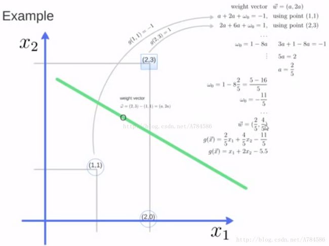
题目：

3. 在cmd中运行如下的Python程序：

from sklearn import svm


x = [[2, 0], [1, 1], [2, 3]]
y = [0, 0, 1]
clf = svm.SVC(kernel = 'linear')
clf.fit(x, y)

print (clf)

# get support vectors
print (clf.support_vectors_)
# get indices of support vectors
print (clf.support_)
# get number of support vectors for each class
print (clf.n_support_)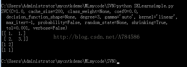

运行效果图：

2.运行一个更复杂的例子并且画图可视化下;

在cmd中运行如下的Python程序：

import numpy as np
import pylab as pl
from sklearn import svm

# we create 40 separable points
X = np.r_[np.random.randn(20, 2) - [2, 2], np.random.randn(20, 2) + [2, 2]]
Y = [0]*20 +[1]*20

#fit the model
clf = svm.SVC(kernel='linear')
clf.fit(X, Y)

# get the separating hyperplane
w = clf.coef_[0]
a = -w[0]/w[1]
xx = np.linspace(-5, 5)
yy = a*xx - (clf.intercept_[0])/w[1]

# plot the parallels to the separating hyperplane that pass through the support vectors
b = clf.support_vectors_[0]
yy_down = a*xx + (b[1] - a*b[0])
b = clf.support_vectors_[-1]
yy_up = a*xx + (b[1] - a*b[0])

print ("w: ", w)
print ("a: ", a)

# print "xx: ", xx
# print "yy: ", yy
print ("support_vectors_: ", clf.support_vectors_)
print ("clf.coef_: ", clf.coef_)

# switching to the generic n-dimensional parameterization of the hyperplan to the 2D-specific equation
# of a line y=a.x +b: the generic w_0x + w_1y +w_3=0 can be rewritten y = -(w_0/w_1) x + (w_3/w_1)


# plot the line, the points, and the nearest vectors to the plane
pl.plot(xx, yy, 'k-')
pl.plot(xx, yy_down, 'k--')
pl.plot(xx, yy_up, 'k--')

pl.scatter(clf.support_vectors_[:, 0], clf.support_vectors_[:, 1],
          s=80, facecolors='none')
pl.scatter(X[:, 0], X[:, 1], c=Y, cmap=pl.cm.Paired)

pl.axis('tight')
pl.show()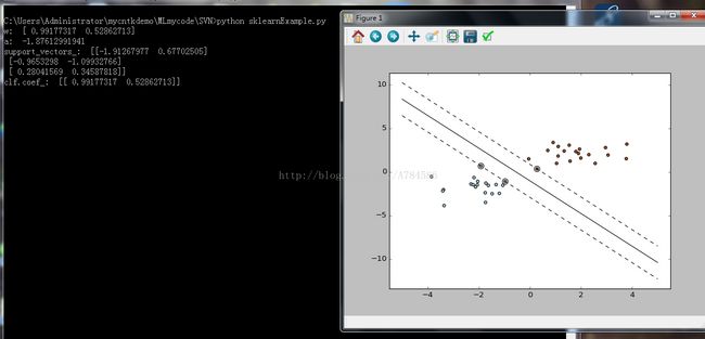

运行效果图如下：

利用SVM处理人脸识别的demo：

在cmd中运行如下的Python程序：

from __future__ import print_function

from time import time
import logging
import matplotlib.pyplot as plt

from sklearn.cross_validation import train_test_split
from sklearn.datasets import fetch_lfw_people
from sklearn.grid_search import GridSearchCV
from sklearn.metrics import classification_report
from sklearn.metrics import confusion_matrix
from sklearn.decomposition import RandomizedPCA
from sklearn.svm import SVC


print(__doc__)

# Display progress logs on stdout
logging.basicConfig(level=logging.INFO, format='%(asctime)s %(message)s')


###############################################################################
# Download the data, if not already on disk and load it as numpy arrays

lfw_people = fetch_lfw_people(min_faces_per_person=70, resize=0.4)

# introspect the images arrays to find the shapes (for plotting)
n_samples, h, w = lfw_people.images.shape

# for machine learning we use the 2 data directly (as relative pixel
# positions info is ignored by this model)
X = lfw_people.data
n_features = X.shape[1]

# the label to predict is the id of the person
y = lfw_people.target
target_names = lfw_people.target_names
n_classes = target_names.shape[0]

print("Total dataset size:")
print("n_samples: %d" % n_samples)
print("n_features: %d" % n_features)
print("n_classes: %d" % n_classes)


###############################################################################
# Split into a training set and a test set using a stratified k fold

# split into a training and testing set
X_train, X_test, y_train, y_test = train_test_split(
    X, y, test_size=0.25)


###############################################################################
# Compute a PCA (eigenfaces) on the face dataset (treated as unlabeled
# dataset): unsupervised feature extraction / dimensionality reduction
n_components = 150

print("Extracting the top %d eigenfaces from %d faces"
      % (n_components, X_train.shape[0]))
t0 = time()
pca = RandomizedPCA(n_components=n_components, whiten=True).fit(X_train)
print("done in %0.3fs" % (time() - t0))

eigenfaces = pca.components_.reshape((n_components, h, w))

print("Projecting the input data on the eigenfaces orthonormal basis")
t0 = time()
X_train_pca = pca.transform(X_train)
X_test_pca = pca.transform(X_test)
print("done in %0.3fs" % (time() - t0))


###############################################################################
# Train a SVM classification model

print("Fitting the classifier to the training set")
t0 = time()
param_grid = {'C': [1e3, 5e3, 1e4, 5e4, 1e5],
              'gamma': [0.0001, 0.0005, 0.001, 0.005, 0.01, 0.1], }
clf = GridSearchCV(SVC(kernel='rbf', class_weight='auto'), param_grid)
clf = clf.fit(X_train_pca, y_train)
print("done in %0.3fs" % (time() - t0))
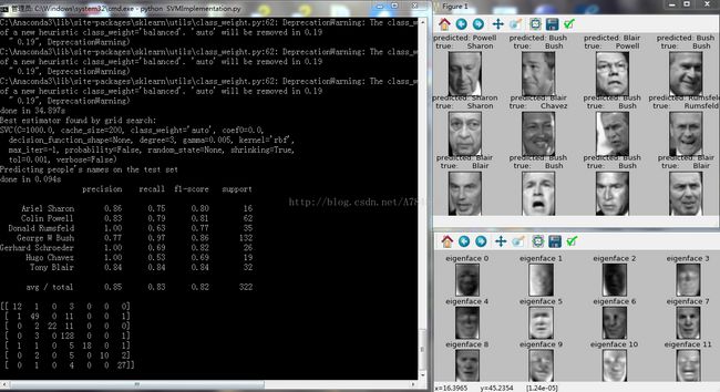
print("Best estimator found by grid search:")
print(clf.best_estimator_)


###############################################################################
# Quantitative evaluation of the model quality on the test set

print("Predicting people's names on the test set")
t0 = time()
y_pred = clf.predict(X_test_pca)
print("done in %0.3fs" % (time() - t0))

print(classification_report(y_test, y_pred, target_names=target_names))
print(confusion_matrix(y_test, y_pred, labels=range(n_classes)))


###############################################################################
# Qualitative evaluation of the predictions using matplotlib

def plot_gallery(images, titles, h, w, n_row=3, n_col=4):
    """Helper function to plot a gallery of portraits"""
    plt.figure(figsize=(1.8 * n_col, 2.4 * n_row))
    plt.subplots_adjust(bottom=0, left=.01, right=.99, top=.90, hspace=.35)
    for i in range(n_row * n_col):
        plt.subplot(n_row, n_col, i + 1)
        plt.imshow(images[i].reshape((h, w)), cmap=plt.cm.gray)
        plt.title(titles[i], size=12)
        plt.xticks(())
        plt.yticks(())


# plot the result of the prediction on a portion of the test set

def title(y_pred, y_test, target_names, i):
    pred_name = target_names[y_pred[i]].rsplit(' ', 1)[-1]
    true_name = target_names[y_test[i]].rsplit(' ', 1)[-1]
    return 'predicted: %s\ntrue:      %s' % (pred_name, true_name)

prediction_titles = [title(y_pred, y_test, target_names, i)
                     for i in range(y_pred.shape[0])]

plot_gallery(X_test, prediction_titles, h, w)

# plot the gallery of the most significative eigenfaces

eigenface_titles = ["eigenface %d" % i for i in range(eigenfaces.shape[0])]
plot_gallery(eigenfaces, eigenface_titles, h, w)

plt.show()

运行效果图：