GBDT回归的python官方例子详解

简单的GBDT调用见官方例子：

方法地址：http://scikit-learn.org/stable/auto_examples/ensemble/plot_gradient_boosting_regression.html#sphx-glr-auto-examples-ensemble-plot-gradient-boosting-regression-py

import numpy as np import matplotlib.pyplot as plt from sklearn import ensemble from sklearn import datasets from sklearn.utils import shuffle from sklearn.metrics import mean_squared_error boston = datasets.load_boston() X, y = shuffle(boston.data, boston.target, random_state = 13 ) X = X.astype(np.float32) offset = int(X.shape[0] * 0.9 ) X_train, y_train = X[:offset], y[:offset] X_test, y_test = X[offset:], y[offset:] params = { ' n_estimators ' : 500 , ' max_depth ' : 4 , ' min_samples_split ' : 2 , ' learning_rate ' : 0.01 , ' loss ' : ' ls ' } clf = ensemble.GradientBoostingRegressor( ** params) clf.fit(X_train, y_train) # 训练 mse = mean_squared_error(y_test, clf.predict(X_test)) # 预测并且计算MSE # print 2.7和3.0版本有区别 print " MSE: %.4f " % mse # compute test set deviance test_score = np.zeros((params[ ' n_estimators ' ],), dtype = np.float64) # 矩阵转化 for i, y_pred in enumerate(clf.staged_predict(X_test)): test_score[i] = clf.loss_(y_test, y_pred) plt.figure(figsize = ( 12 , 6 )) plt.subplot( 1 , 2 , 1 ) plt.title( ' Deviance ' ) plt.plot(np.arange(params[ ' n_estimators ' ]) + 1 , clf.train_score_, ' b- ' , label = ' Training Set Deviance ' ) plt.plot(np.arange(params[ ' n_estimators ' ]) + 1 , test_score, ' r- ' , label = ' Test Set Deviance ' ) plt.legend(loc = ' upper right ' ) plt.xlabel( ' Boosting Iterations ' ) plt.ylabel( ' Deviance ' ) # Plot feature importance feature_importance = clf.feature_importances_ # make importances relative to max importance feature_importance = 100.0 * (feature_importance / feature_importance.max()) sorted_idx = np.argsort(feature_importance) pos = np.arange(sorted_idx.shape[0]) + . 5 plt.subplot( 1 , 2 , 2 ) plt.barh(pos, feature_importance[sorted_idx], align = ' center ' ) plt.yticks(pos, boston.feature_names[sorted_idx]) plt.xlabel( ' Relative Importance ' ) plt.title( ' Variable Importance ' ) plt.show()

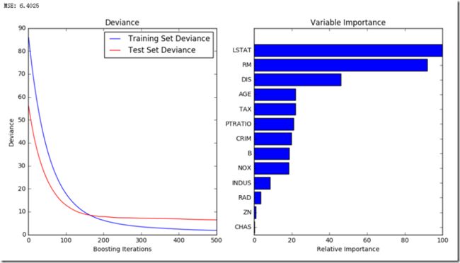
输出：

 

结论：LSTAT>RM>DIS………

 

房产的数据结构：

- CRIM     per capita crime rate by town
- ZN       proportion of residential land zoned for lots over 25,000 sq.ft.
- INDUS    proportion of non-retail business acres per town
- CHAS     Charles River dummy variable (= 1 if tract bounds river; 0 otherwise)
- NOX      nitric oxides concentration (parts per 10 million)
- RM       average number of rooms per dwelling
- AGE      proportion of owner-occupied units built prior to 1940
- DIS      weighted distances to five Boston employment centres
- RAD      index of accessibility to radial highways
- TAX      full-value property-tax rate per $10,000
- PTRATIO  pupil-teacher ratio by town
- B        1000(Bk - 0.63)^2 where Bk is the proportion of blacks by town
- LSTAT    % lower status of the population
- MEDV     Median value of owner-occupied homes in $1000's

 

源代码读取csv文件方法详解：

def load_boston():
    """Load and return the boston house-prices dataset (regression).

    ==============     ==============
    Samples total                 506
    Dimensionality                 13
    Features           real, positive
    Targets             real 5. - 50.
    ==============     ==============

    Returns
    -------
    data : Bunch
        Dictionary-like object, the interesting attributes are:
        'data', the data to learn, 'target', the regression targets,
        and 'DESCR', the full description of the dataset.

    Examples
    --------
    >>> from sklearn.datasets import load_boston
    >>> boston = load_boston()
    >>> print(boston.data.shape)
    (506, 13)
    """
    module_path = dirname(__file__)

    fdescr_name = join(module_path, 'descr', 'boston_house_prices.rst')
    with open(fdescr_name) as f:  #with用法可以自动关闭，读取文件声明
        descr_text = f.read()

    data_file_name = join(module_path, 'data', 'boston_house_prices.csv')
    with open(data_file_name) as f:
        data_file = csv.reader(f)  #csv读取文件，获得迭代器
        temp = next(data_file)     #读取文件头，获得总行数和字段名
        n_samples = int(temp[0])
        n_features = int(temp[1])
        data = np.empty((n_samples, n_features)) #建立矩阵
        target = np.empty((n_samples,))
        temp = next(data_file)  # names of features
        feature_names = np.array(temp)

        for i, d in enumerate(data_file):  #一行一行通过迭代器读取文件设置到矩阵中
            data[i] = np.asarray(d[:-1], dtype=np.float)
            target[i] = np.asarray(d[-1], dtype=np.float)

    return Bunch(data=data,
                 target=target,
                 # last column is target value
                 feature_names=feature_names[:-1],
                 DESCR=descr_text)

 

方法说明：

1、with是python的一种用法，可以自动关闭对应的资源

2、next(iterator[, default])  迭代器遍历方法

3、reader(csvfile, dialect='excel', **fmtparams) ：返回一个迭代器

Return a reader object which will iterate over lines in the given csvfile.

 

 

 

类的主要方法介绍：

构造函数：
loss
learning_rate
n_estimators
max_depth
criterion
min_samples_split
min_samples_leaf
min_weight_fraction_leaf
subsample
max_features
max_leaf_nodes
min_impurity_split
alpha
init
verbose
warm_start
random_state
presort

属性

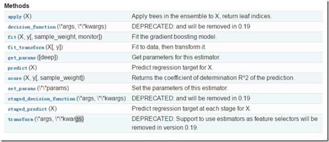
方法
feature_importances_ ：重要的特性
oob_improvement_：
train_score_ ：训练分数
loss_ ：损失函数
`init` : 评估期
estimators_ : ndarray of DecisionTreeRegressor, shape = [n_estimators, 1]

方法：

 

后续待补充详细参数说明