深入浅出python机器学习_8.2_神经网络的原理及应用

import numpy as np

import matplotlib.pyplot as plt

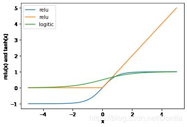
line=np.linspace(-5,5,200)

plt.plot(line,np.tanh(line),label='relu')

plt.plot(line,np.maximum(line,0),label='relu')

# a=[]
# for i in line:
#     j=1/(1+np.exp(-i))
#     a.append(j)

plt.plot(line,1/(1+np.exp(-line)),label='logitic')

plt.legend(loc='best')

plt.xlabel('x')

plt.ylabel('relu(x) and tanh(x)')

plt.show()

from sklearn.neural_network import MLPClassifier

from sklearn.datasets import load_wine

from sklearn.model_selection import train_test_split

wine=load_wine()

print('打印wine:\n',wine,'\n')

print('打印wine.data.shape',wine.data.shape,'\n')

打印wine:
 {'data': array([[1.423e+01, 1.710e+00, 2.430e+00, ..., 1.040e+00, 3.920e+00,
        1.065e+03],
       [1.320e+01, 1.780e+00, 2.140e+00, ..., 1.050e+00, 3.400e+00,
        1.050e+03],
       [1.316e+01, 2.360e+00, 2.670e+00, ..., 1.030e+00, 3.170e+00,
        1.185e+03],
       ...,
       [1.327e+01, 4.280e+00, 2.260e+00, ..., 5.900e-01, 1.560e+00,
        8.350e+02],
       [1.317e+01, 2.590e+00, 2.370e+00, ..., 6.000e-01, 1.620e+00,
        8.400e+02],
       [1.413e+01, 4.100e+00, 2.740e+00, ..., 6.100e-01, 1.600e+00,
        5.600e+02]]), 'target': array([0, 0, 0, 0, 0, 0, 0, 0, 0, 0, 0, 0, 0, 0, 0, 0, 0, 0, 0, 0, 0, 0,
       0, 0, 0, 0, 0, 0, 0, 0, 0, 0, 0, 0, 0, 0, 0, 0, 0, 0, 0, 0, 0, 0,
       0, 0, 0, 0, 0, 0, 0, 0, 0, 0, 0, 0, 0, 0, 0, 1, 1, 1, 1, 1, 1, 1,
       1, 1, 1, 1, 1, 1, 1, 1, 1, 1, 1, 1, 1, 1, 1, 1, 1, 1, 1, 1, 1, 1,
       1, 1, 1, 1, 1, 1, 1, 1, 1, 1, 1, 1, 1, 1, 1, 1, 1, 1, 1, 1, 1, 1,
       1, 1, 1, 1, 1, 1, 1, 1, 1, 1, 1, 1, 1, 1, 1, 1, 1, 1, 1, 1, 2, 2,
       2, 2, 2, 2, 2, 2, 2, 2, 2, 2, 2, 2, 2, 2, 2, 2, 2, 2, 2, 2, 2, 2,
       2, 2, 2, 2, 2, 2, 2, 2, 2, 2, 2, 2, 2, 2, 2, 2, 2, 2, 2, 2, 2, 2,
       2, 2]), 'target_names': array(['class_0', 'class_1', 'class_2'], dtype='

# 最外维全取, 次外维取下标0和1
X=wine.data[:,:2]

print('打印X:\n',X,'\n')

print('打印X.shape:\n',X.shape,'\n')

y=wine.target

X_train,X_test,y_train,y_test=train_test_split(X,y,random_state=0)

print('X_train.shape:\n',X_train.shape,'\n')

print('X_test.shape:\n',X_test.shape,'\n')

print('y_train.shape:\n',y_train.shape,'\n')

print('y_test.shape:\n',y_test.shape,'\n')

打印X:
 [[14.23  1.71]
 [13.2   1.78]
 [13.16  2.36]
 [14.37  1.95]
 [13.24  2.59]
 [14.2   1.76]
 [14.39  1.87]
 [14.06  2.15]
 [14.83  1.64]
 [13.86  1.35]
 [14.1   2.16]
 [14.12  1.48]
 [13.75  1.73]
 [14.75  1.73]
 [14.38  1.87]
 [13.63  1.81]
 [14.3   1.92]
 [13.83  1.57]
 [14.19  1.59]
 [13.64  3.1 ]
 [14.06  1.63]
 [12.93  3.8 ]
 [13.71  1.86]
 [12.85  1.6 ]
 [13.5   1.81]
 [13.05  2.05]
 [13.39  1.77]
 [13.3   1.72]
 [13.87  1.9 ]
 [14.02  1.68]
 [13.73  1.5 ]
 [13.58  1.66]
 [13.68  1.83]
 [13.76  1.53]
 [13.51  1.8 ]
 [13.48  1.81]
 [13.28  1.64]
 [13.05  1.65]
 [13.07  1.5 ]
 [14.22  3.99]
 [13.56  1.71]
 [13.41  3.84]
 [13.88  1.89]
 [13.24  3.98]
 [13.05  1.77]
 [14.21  4.04]
 [14.38  3.59]
 [13.9   1.68]
 [14.1   2.02]
 [13.94  1.73]
 [13.05  1.73]
 [13.83  1.65]
 [13.82  1.75]
 [13.77  1.9 ]
 [13.74  1.67]
 [13.56  1.73]
 [14.22  1.7 ]
 [13.29  1.97]
 [13.72  1.43]
 [12.37  0.94]
 [12.33  1.1 ]
 [12.64  1.36]
 [13.67  1.25]
 [12.37  1.13]
 [12.17  1.45]
 [12.37  1.21]
 [13.11  1.01]
 [12.37  1.17]
 [13.34  0.94]
 [12.21  1.19]
 [12.29  1.61]
 [13.86  1.51]
 [13.49  1.66]
 [12.99  1.67]
 [11.96  1.09]
 [11.66  1.88]
 [13.03  0.9 ]
 [11.84  2.89]
 [12.33  0.99]
 [12.7   3.87]
 [12.    0.92]
 [12.72  1.81]
 [12.08  1.13]
 [13.05  3.86]
 [11.84  0.89]
 [12.67  0.98]
 [12.16  1.61]
 [11.65  1.67]
 [11.64  2.06]
 [12.08  1.33]
 [12.08  1.83]
 [12.    1.51]
 [12.69  1.53]
 [12.29  2.83]
 [11.62  1.99]
 [12.47  1.52]
 [11.81  2.12]
 [12.29  1.41]
 [12.37  1.07]
 [12.29  3.17]
 [12.08  2.08]
 [12.6   1.34]
 [12.34  2.45]
 [11.82  1.72]
 [12.51  1.73]
 [12.42  2.55]
 [12.25  1.73]
 [12.72  1.75]
 [12.22  1.29]
 [11.61  1.35]
 [11.46  3.74]
 [12.52  2.43]
 [11.76  2.68]
 [11.41  0.74]
 [12.08  1.39]
 [11.03  1.51]
 [11.82  1.47]
 [12.42  1.61]
 [12.77  3.43]
 [12.    3.43]
 [11.45  2.4 ]
 [11.56  2.05]
 [12.42  4.43]
 [13.05  5.8 ]
 [11.87  4.31]
 [12.07  2.16]
 [12.43  1.53]
 [11.79  2.13]
 [12.37  1.63]
 [12.04  4.3 ]
 [12.86  1.35]
 [12.88  2.99]
 [12.81  2.31]
 [12.7   3.55]
 [12.51  1.24]
 [12.6   2.46]
 [12.25  4.72]
 [12.53  5.51]
 [13.49  3.59]
 [12.84  2.96]
 [12.93  2.81]
 [13.36  2.56]
 [13.52  3.17]
 [13.62  4.95]
 [12.25  3.88]
 [13.16  3.57]
 [13.88  5.04]
 [12.87  4.61]
 [13.32  3.24]
 [13.08  3.9 ]
 [13.5   3.12]
 [12.79  2.67]
 [13.11  1.9 ]
 [13.23  3.3 ]
 [12.58  1.29]
 [13.17  5.19]
 [13.84  4.12]
 [12.45  3.03]
 [14.34  1.68]
 [13.48  1.67]
 [12.36  3.83]
 [13.69  3.26]
 [12.85  3.27]
 [12.96  3.45]
 [13.78  2.76]
 [13.73  4.36]
 [13.45  3.7 ]
 [12.82  3.37]
 [13.58  2.58]
 [13.4   4.6 ]
 [12.2   3.03]
 [12.77  2.39]
 [14.16  2.51]
 [13.71  5.65]
 [13.4   3.91]
 [13.27  4.28]
 [13.17  2.59]
 [14.13  4.1 ]] 

打印X.shape:
 (178, 2) 

X_train.shape:
 (133, 2) 

X_test.shape:
 (45, 2) 

y_train.shape:
 (133,) 

y_test.shape:
 (45,) 

#  - 'lbfgs' is an optimizer in the family of quasi-Newton methods.
# “lbfgs”是准牛顿方法家族中的一个优化器。
# 默认隐藏层为1层,节点为100个

mlp=MLPClassifier(solver='lbfgs')

mlp.fit(X_train,y_train)

MLPClassifier(activation='relu', alpha=0.0001, batch_size='auto', beta_1=0.9,
              beta_2=0.999, early_stopping=False, epsilon=1e-08,
              hidden_layer_sizes=(100,), learning_rate='constant',
              learning_rate_init=0.001, max_iter=200, momentum=0.9,
              n_iter_no_change=10, nesterovs_momentum=True, power_t=0.5,
              random_state=None, shuffle=True, solver='lbfgs', tol=0.0001,
              validation_fraction=0.1, verbose=False, warm_start=False)

from matplotlib.colors import ListedColormap

cmap_light=ListedColormap(['#FFAAAA','#AAFFAA','#AAAAFF'])

cmap_bold=ListedColormap(['#FF0000','#00FF00','0000FF'])

print('打印cmap_light:\n',cmap_light,'\n')

print('打印cmap_light的类型:\n',type(cmap_light),'\n')

x_min,x_max=X_train[:,0].min()-1,X_train[:,0].max()+1

y_min,y_max=X_train[:,1].min()-1,X_train[:,1].max()+1

xx,yy=np.meshgrid(np.arange(x_min,x_max,.02),np.arange(y_min,y_max,.02))

Z=mlp.predict(np.c_[xx.ravel(),yy.ravel()])

Z=Z.reshape(xx.shape)

plt.figure()

plt.pcolormesh(xx,yy,Z,cmap=cmap_light)

# plt.scatter(xx,yy,c=Z,cmap=cmap_light)

plt.scatter(X[:,0],X[:,1],c=y,edgecolors='k',s=60)

plt.xlim(xx.min(),xx.max())

plt.ylim(yy.min(),yy.max())

plt.title('MLPClassifier:solver=lbfgs')

plt.show()

打印cmap_light:
  

打印cmap_light的类型:
  

# 将隐藏层节点数设置为10

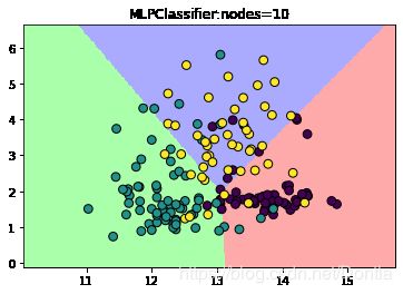
mlp_20=MLPClassifier(solver='lbfgs',hidden_layer_sizes=[10])

mlp_20.fit(X_train,y_train)

Z1=mlp_20.predict(np.c_[xx.ravel(),yy.ravel()])

Z1=Z1.reshape(xx.shape)

plt.figure()

plt.pcolormesh(xx,yy,Z1,cmap=cmap_light)


plt.scatter(X[:,0],X[:,1],c=y,edgecolors='k',s=60)

plt.xlim(xx.min(),xx.max())

plt.ylim(yy.min(),yy.max())

plt.title('MLPClassifier:nodes=10')

plt.show()

# 将隐藏层层数设置为2

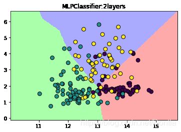
mlp_2L=MLPClassifier(solver='lbfgs',hidden_layer_sizes=[10,10])

mlp_2L.fit(X_train,y_train)

Z1=mlp_2L.predict(np.c_[xx.ravel(),yy.ravel()])

Z1=Z1.reshape(xx.shape)

plt.figure()

plt.pcolormesh(xx,yy,Z1,cmap=cmap_light)


plt.scatter(X[:,0],X[:,1],c=y,edgecolors='k',s=60)

plt.xlim(xx.min(),xx.max())

plt.ylim(yy.min(),yy.max())

plt.title('MLPClassifier:2layers')

plt.show()

# 设置激活函数为tanh

mlp_tanh=MLPClassifier(solver='lbfgs',hidden_layer_sizes=[10,10],activation='tanh')

mlp_tanh.fit(X_train,y_train)

Z2=mlp_tanh.predict(np.c_[xx.ravel(),yy.ravel()])

Z2=Z2.reshape(xx.shape)

plt.figure()

plt.pcolormesh(xx,yy,Z2,cmap=cmap_light)


plt.scatter(X[:,0],X[:,1],c=y,edgecolors='k',s=60)

plt.xlim(xx.min(),xx.max())

plt.ylim(yy.min(),yy.max())

plt.title('MLPClassifier:2layers with tanh')

plt.show()

# 增大模型的alpha参数,减小模型的复杂度

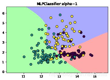
mlp_alpha=MLPClassifier(solver='lbfgs',hidden_layer_sizes=[10,10],activation='tanh',alpha=1)

mlp_alpha.fit(X_train,y_train)

Z3=mlp_alpha.predict(np.c_[xx.ravel(),yy.ravel()])

Z3=Z3.reshape(xx.shape)

plt.figure()

plt.pcolormesh(xx,yy,Z2,cmap=cmap_light)


plt.scatter(X[:,0],X[:,1],c=y,edgecolors='k',s=60)

plt.xlim(xx.min(),xx.max())

plt.ylim(yy.min(),yy.max())

plt.title('MLPClassifier:alpha=1')

plt.show()