周志华《机器学习》Ch3. 线性模型：对数几率回归的python实现

理论

        “对数几率模型”就是常说的Logistic回归，是一个经典的线性模型。考虑二分类任务，其输出标记，而线性回归模型产生的预测值是连续分布的实数，需要一个阶跃函数将连续值映射为离散二值。用一个对数几率函数近似阶跃函数，得到。从而y和1-y可以分别视为类后验概率和，简记为和。

     训练时，用极大似然法估计模型参数和. 对给定的数据集，对数几率模型最大化对数似然函数. 令, , 似然函数可重写为.

        上述似然函数可以用经典的优化算法如梯度下降法、牛顿法求解。以牛顿法为例，其第t+1轮迭代解的更新公式为, 其中， .

代码

# -*- coding: utf-8 -*-
"""
Logistic Regression
From 'Machine Learning, Zhihua Zhou'
Model: P69 problem 3.3
        linear model
        Newton Method
Dataset: P89 watermelon_3.0a (watermelon_3.0a.npy)

@author: weiyx15
"""

import numpy as np
import matplotlib.pyplot as plt

class Logistic:
    def load_data(self, filename):
        dic = np.load(filename)
        self.x = dic['arr_0']
        self.y = dic['arr_1']
        self.m = self.x.shape[0]
        self.d = self.x.shape[1]
        
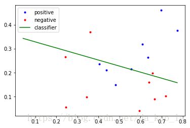
    def plot_data(self):
        x1 = self.x[np.where(self.y==1),:]
        x1 = x1.reshape((x1.shape[1], x1.shape[2]))
        x0 = self.x[np.where(self.y==0),:]
        x0 = x0.reshape((x0.shape[1], x0.shape[2]))
        plt.plot(x1[:,0], x1[:,1], 'b.')
        plt.plot(x0[:,0], x0[:,1], 'r.')
        x0min = x0.min()
        x1min = x1.min()
        xmin = min(x0min, x1min)
        x0max = x0.max()
        x1max = x1.max()
        xmax = max(x0max, x1max)
        xs = np.linspace(xmin, xmax, 100)
        beta = self.beta.reshape((self.beta.shape[1],))
        ys = -beta[0]/beta[1]*xs - beta[2]/beta[1]
        plt.plot(xs, ys, 'g')
        plt.legend(['positive', 'negative', 'classifier'])
        
    def __init__(self):
        self.load_data('watermelon_3.0a.npz')
    
    def calculate_derivative(self, beta):
        pLpB = np.zeros((self.d+1,))
        pLpB2 = np.zeros((self.d+1, self.d+1))
        pLpB2 = np.mat(pLpB2)
        ones = np.ones((self.m,1))
        x1 = np.concatenate((self.x, ones), axis=1)
        for i in range(self.m):
            myexp = np.exp(np.dot(beta, x1[i]))
            p1 = myexp / (1+myexp)
            x1i = np.mat(x1[i])
            pLpB = pLpB - (self.y[i] - p1)*x1[i]
            addi = np.dot(x1i.T, x1i)
            addi = np.multiply(addi, p1*(1-p1))
            pLpB2 = pLpB2 + addi
        return pLpB, pLpB2
    
    def train(self):
        self.beta = np.ones((self.d+1,))
        p_beta = np.zeros((self.d+1,))
        while np.linalg.norm(self.beta-p_beta) > 1e-3:
            p_beta = self.beta
            pLpB, pLpB2 = self.calculate_derivative(p_beta)
            self.beta = p_beta - np.dot(pLpB2.I, pLpB).getA()
    
    def classify(self, xt):
        xt.append(1)
        xt = np.array(xt)
        myexp = np.exp(np.dot(self.beta.reshape((self.beta.size,)), xt))
        p1 = myexp / (1+myexp)
        if p1 > .5:
            return 1
        else:
            return 0

if __name__ == '__main__':
    lg = Logistic()
    lg.train()
    ans = lg.classify([.555, .354])
    lg.plot_data()

结果