TF/04_Support_Vector_Machines/04_Working_with_Kernels

Working with Kernels

Linear SVMs are very powerful. But sometimes the data are not very linear. To this end, we can use the ‘kernel trick’ to map our data into a higher dimensional space, where it may be linearly separable. Doing this allows us to separate out non-linear classes. See the below example.

If we attempt to separate the below circular-ring shaped classes with a standard linear SVM, we fail.

But if we separate it with a Gaussian-RBF kernel, we can find a linear separator in a higher dimension that works a lot better.

# 04_svm_kernels.py
# Illustration of Various Kernels
#----------------------------------
#
# This function wll illustrate how to
# implement various kernels in TensorFlow.
#
# Linear Kernel:
# K(x1, x2) = t(x1) * x2
#
# Gaussian Kernel (RBF):
# K(x1, x2) = exp(-gamma * abs(x1 - x2)^2)

import matplotlib.pyplot as plt
import numpy as np
import tensorflow as tf
from sklearn import datasets
from tensorflow.python.framework import ops
ops.reset_default_graph()

# Create graph
#修改位置
config = tf.ConfigProto(allow_soft_placement= True, log_device_placement= True)
sess = tf.Session(config = config)
# Create graph
#sess = tf.Session()

# Generate non-lnear data
(x_vals, y_vals) = datasets.make_circles(n_samples=350, factor=.5, noise=.1)
y_vals = np.array([1 if y==1 else -1 for y in y_vals])
class1_x = [x[0] for i,x in enumerate(x_vals) if y_vals[i]==1]
class1_y = [x[1] for i,x in enumerate(x_vals) if y_vals[i]==1]
class2_x = [x[0] for i,x in enumerate(x_vals) if y_vals[i]==-1]
class2_y = [x[1] for i,x in enumerate(x_vals) if y_vals[i]==-1]

# Declare batch size
batch_size = 350

# Initialize placeholders
x_data = tf.placeholder(shape=[None, 2], dtype=tf.float32)
y_target = tf.placeholder(shape=[None, 1], dtype=tf.float32)
prediction_grid = tf.placeholder(shape=[None, 2], dtype=tf.float32)

# Create variables for svm
b = tf.Variable(tf.random_normal(shape=[1,batch_size]))

# Apply kernel
# Linear Kernel
# my_kernel = tf.matmul(x_data, tf.transpose(x_data))

# Gaussian (RBF) kernel
gamma = tf.constant(-50.0)
dist = tf.reduce_sum(tf.square(x_data), 1)
dist = tf.reshape(dist, [-1,1])
sq_dists = tf.add(tf.subtract(dist, tf.multiply(2., tf.matmul(x_data, tf.transpose(x_data)))), tf.transpose(dist))
my_kernel = tf.exp(tf.multiply(gamma, tf.abs(sq_dists)))

# Compute SVM Model
first_term = tf.reduce_sum(b)
b_vec_cross = tf.matmul(tf.transpose(b), b)
y_target_cross = tf.matmul(y_target, tf.transpose(y_target))
second_term = tf.reduce_sum(tf.multiply(my_kernel, tf.multiply(b_vec_cross, y_target_cross)))
loss = tf.negative(tf.subtract(first_term, second_term))

# Create Prediction Kernel
# Linear prediction kernel
# my_kernel = tf.matmul(x_data, tf.transpose(prediction_grid))

# Gaussian (RBF) prediction kernel
rA = tf.reshape(tf.reduce_sum(tf.square(x_data), 1),[-1,1])
rB = tf.reshape(tf.reduce_sum(tf.square(prediction_grid), 1),[-1,1])
pred_sq_dist = tf.add(tf.subtract(rA, tf.multiply(2., tf.matmul(x_data, tf.transpose(prediction_grid)))), tf.transpose(rB))
pred_kernel = tf.exp(tf.multiply(gamma, tf.abs(pred_sq_dist)))

prediction_output = tf.matmul(tf.multiply(tf.transpose(y_target),b), pred_kernel)
prediction = tf.sign(prediction_output-tf.reduce_mean(prediction_output))
accuracy = tf.reduce_mean(tf.cast(tf.equal(tf.squeeze(prediction), tf.squeeze(y_target)), tf.float32))

# Declare optimizer
my_opt = tf.train.GradientDescentOptimizer(0.002)
train_step = my_opt.minimize(loss)

# Initialize variables
init = tf.global_variables_initializer()
sess.run(init)

# Training loop
loss_vec = []
batch_accuracy = []
for i in range(1000):
    rand_index = np.random.choice(len(x_vals), size=batch_size)
    rand_x = x_vals[rand_index]
    rand_y = np.transpose([y_vals[rand_index]])
    sess.run(train_step, feed_dict={x_data: rand_x, y_target: rand_y})

    temp_loss = sess.run(loss, feed_dict={x_data: rand_x, y_target: rand_y})
    loss_vec.append(temp_loss)

    acc_temp = sess.run(accuracy, feed_dict={x_data: rand_x,
                                             y_target: rand_y,
                                             prediction_grid:rand_x})
    batch_accuracy.append(acc_temp)

    if (i+1)%250==0:
        print('Step #' + str(i+1))
        print('Loss = ' + str(temp_loss))

# Create a mesh to plot points in
x_min, x_max = x_vals[:, 0].min() - 1, x_vals[:, 0].max() + 1
y_min, y_max = x_vals[:, 1].min() - 1, x_vals[:, 1].max() + 1
xx, yy = np.meshgrid(np.arange(x_min, x_max, 0.02),
                     np.arange(y_min, y_max, 0.02))
grid_points = np.c_[xx.ravel(), yy.ravel()]
[grid_predictions] = sess.run(prediction, feed_dict={x_data: rand_x,
                                                   y_target: rand_y,
                                                   prediction_grid: grid_points})
grid_predictions = grid_predictions.reshape(xx.shape)

# Plot points and grid
plt.contourf(xx, yy, grid_predictions, cmap=plt.cm.Paired, alpha=0.8)
plt.plot(class1_x, class1_y, 'ro', label='Class 1')
plt.plot(class2_x, class2_y, 'kx', label='Class -1')
plt.title('Gaussian SVM Results')
plt.xlabel('x')
plt.ylabel('y')
plt.legend(loc='lower right')
plt.ylim([-1.5, 1.5])
plt.xlim([-1.5, 1.5])
plt.show()

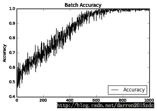
# Plot batch accuracy
plt.plot(batch_accuracy, 'k-', label='Accuracy')
plt.title('Batch Accuracy')
plt.xlabel('Generation')
plt.ylabel('Accuracy')
plt.legend(loc='lower right')
plt.show()

# Plot loss over time
plt.plot(loss_vec, 'k-')
plt.title('Loss per Generation')
plt.xlabel('Generation')
plt.ylabel('Loss')
plt.show()

Step #250
Loss = 49.561
Step #500
Loss = -5.57512
Step #750
Loss = -11.3843
Step #1000
Loss = -11.6753